python可以小程序开发吗,python能开发应用程序吗-程序员宅基地
技术标签: 人工智能
大家好,给大家分享一下python可以用来开发小程序吗,很多人还不知道这一点。下面详细解释一下。现在让我们来看看!

用python做一个简单软件
前言
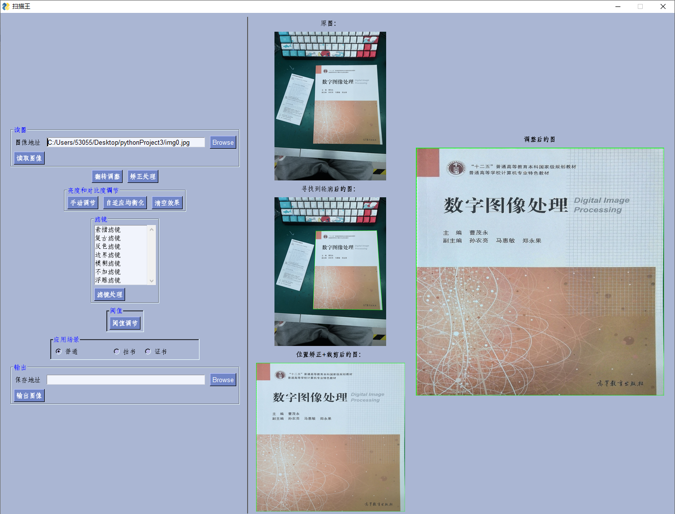
这是一个课设,用python做一个扫描王软件
我主要做的GUI部分,记录分享一下。也是第一次用python做小软件,python的方便果然是名不虚传
遇到问题
1.python版本
下载了python3.7的编译器
由于最终软件要在win7上运行,即32位的,因此下载了python3.7的32位
打包后遇到问题:w10打包的不能在w7上运行----->下载python32位的解释器
在w10执行python代码,参考博客: https://blog.csdn.net/qq_27280237/article/details/84644900
2.opencv降级
参考博客: https://www.cnblogs.com/guobin-/p/10842486.html
3.安装打包软件pyinstaller
参考博客: https://blog.csdn.net/Nire_Yeyu/article/details/104683888/
https://blog.csdn.net/Nire_Yeyu/article/details/104683888/
https://www.cnblogs.com/xbblogs/p/9682708.html
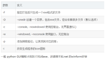
##最终打包代码
pyinstaller -F -w -i 图片名.ico  文件名.py
4.输出的图片没法保存
有中文路径
软件效果
python代码
1.GUI部分
import PySimpleGUI as sg
import PIL.Image
import scanner_doee2
import cv2
import os

import numpy as np

import other
from other import convert_to_bytes


from tkinter import *


# 全局变量
mp_path = ['读取图像','原图处理','滤镜']
mp_key = ['原图处理', '图像翻转', '寻找轮廓','读取图像','img0']
choices = ('素描滤镜','复古滤镜','反色滤镜','边界滤镜', '模糊滤镜','不加滤镜','浮雕滤镜')
#缓存图片标号
# 原图/翻转后的图片  0
# 圈出轮廓的图 10
# 透视变换后 11
# 调整亮度和对比度后的图 2
# 添加滤镜后的图 3

sg.theme('Light Blue 2')
layout1 = [
            [sg.Frame(layout=[
                [sg.Text('图像地址'), sg.Input(key='path_in'), sg.FileBrowse()],
                [sg.Button('读取图像')]
            ], title='读图',title_color='blue')],

          [sg.Button('翻转调整'),sg.Button('矫正处理')],

            [sg.Frame(layout=[
                [sg.Button('手动调节'), sg.Button('自适应均衡化'), sg.Button('清空效果')],
            ], title='亮度和对比度调节',title_color='blue')],

           [sg.Frame(layout = [
                    [sg.Listbox(choices, size=(15, len(choices)), key='filter')],
                    [sg.Button('滤镜处理')]
                                 ],  title='滤镜', title_color='blue') ],

           [sg.Frame(layout=[
               [sg.Button('阈值调节')]],
               title='阈值', title_color='blue', relief=sg.RELIEF_SUNKEN, tooltip='Use these to set flags')],

          [sg.Frame(layout=[
                        [sg.Radio('普通', "RADIO1",key='普通', default=True, size=(10, 1)), sg.Radio('拍书', "RADIO1",key='拍书'),sg.Radio('证书', "RADIO1", key='证件',default=False, size=(10, 1))]],
                        title='应用场景', title_color='blue', relief=sg.RELIEF_SUNKEN, tooltip='Use these to set flags')],


         [sg.Frame(layout=[
            [sg.Text('保存地址'), sg.Input(key='path_out'),sg.FolderBrowse(target='path_out')],
            [sg.Button('输出图像')]
            ], title='输出',title_color='blue')],

]
layout2 = [[sg.Text('原图:')],
              [sg.Image(key='img0',size=(300,300))],

           [sg.Text('寻找到轮廓后的图:')],
           [sg.Image(key='img10',  size=(300, 300))],

            [sg.Text('位置矫正+裁剪后的图:')],
              [sg.Image(key='img11',size=(300, 300))]
           ]
layout3=[ [sg.Text('调整后的图')],
              [sg.Image(key='img2',size=(500,500))]
          ]


layout = [[sg.Column(layout1, element_justification='c'), sg.VSeperator(),sg.Column(layout2, element_justification='c'),sg.Column(layout3, element_justification='c')]]
window = sg.Window('扫描王', layout)


while (True):
    event, values = window.read()
    if event !=None:
        print(event,values)

    if event =='读取图像':
      path_in = values['path_in']
      path_save=os.path.dirname(path_in)
      img0=cv2.imread(path_in)
      print(path_save)
      scanner_doee2.varible(path_save)

      # orig =  img0  #备份原图
      # 重新设置图片的大小,以便对其进行处理:选择最佳维度,以便重要内容不会丢失
      # img0 = cv2.resize(img0, (1500, 880))
      cv2.imwrite(path_save+'/img0.jpg',img0)

      window['img0'].update(data=convert_to_bytes(path_in, (300,300)))


    if event =='翻转调整':
        img0=np.rot90(img0)
        cv2.imwrite(path_save + '/img0.jpg', img0)
        window['img0'].update(data=convert_to_bytes(path_save+'/img0.jpg', (300, 300)))

    if event=='矫正处理':
        img1=scanner_doee2.solve(img0)
        img2=img1
        img3=img1
        window['img10'].update(data=convert_to_bytes(path_save+'/img10.jpg', resize=(300,300)))
        window['img11'].update(data=convert_to_bytes(path_save+'/img11.jpg', resize=(300,300)))

    if event=='清空效果':
        img2=img1
        cv2.imwrite(path_save + '/img2.jpg', img2)
        window['img2'].update(data=convert_to_bytes(path_save+'/img2.jpg', resize=(500,500)))


    if event=='手动调节':
        img2=scanner_doee2.light(img2)
        cv2.imwrite(path_save + '/img2.jpg', img2)
        window['img2'].update(data=convert_to_bytes(path_save+'/img2.jpg', resize=(500,500)))

    if event=='自适应均衡化':
        img2=scanner_doee2.autoEqualHistColor(img2)
        cv2.imwrite(path_save + '/img2.jpg', img2)
        window['img2'].update(data=convert_to_bytes(path_save+'/img2.jpg', resize=(500,500)))

    if event=='滤镜处理':
        img3=img2
        ss=values['filter']
        print(ss,ss[0])
        if ss[0]=='复古滤镜':
            img3 = scanner_doee2.mirror2(img2)
        elif ss[0]=='素描滤镜':
            print(ss)
            img3 = scanner_doee2.mirror1(img2)
        elif ss[0] == '反色滤镜':
            print(ss)
            img3 = scanner_doee2.mirror3(img2)
        elif ss[0] == '边界滤镜':
            img3 = scanner_doee2.mirror4(img2)
        elif ss[0] == '浮雕滤镜':
            img3 = scanner_doee2.mirror5(img2,1)
        elif ss[0] == '模糊滤镜':
            img3 = scanner_doee2.mirror5(img2,2)
        elif ss[0]=='不加滤镜':
            img3=img2

        cv2.imwrite(path_save + '/img2.jpg', img3)
        window['img2'].update(data=convert_to_bytes(path_save + '/img2.jpg', resize=(500, 500)))

    if event=='阈值调节':
        img4=img2
        img4=scanner_doee2.yuzhi(img2)
        cv2.imwrite(path_save + '/img2.jpg', img4)
        window['img2'].update(data=convert_to_bytes(path_save + '/img2.jpg', resize=(500, 500)))

    if event=='输出图像':
        img5=cv2.imread(path_save + '/img2.jpg')
        h,w,c=img5.shape
        # A4 297*210mm
        # B5 250*176
        # 身份证 54*85.6

        if values['拍书']==True:
            scale = min(h/250,  w/176)
            img5=cv2.resize(img5,(int(176* scale), int(250* scale)))

        elif values['证件']==True:
            scale = min(h/54,  w/85.6)
            img5=cv2.resize(img5,(int(85.6* scale), int(54* scale)))

        elif values['普通']==True:
            img5 = cv2.imread(path_save + '/img2.jpg')

        cv2.imshow('output',img5)

        path_out=values['path_out']
        cv2.imwrite( path_out+ '/out.jpg', img5)
        # cv2.imwrite(path_save + '/img2.jpg', img5)


    if event == sg.WIN_CLOSED or event == 'Exit':
        break
2.算法部分
import cv2
import numpy as np
from math import sqrt
import cmath
from PIL import Image, ImageFilter
path_save='yes'
def varible(ss):
    global path_save
    path_save=ss
    print(path_save)

def rectify(h):
    h = h.reshape((4,2))   #改变数组的形状,变成4*2形状的数组
    hnew = np.zeros((4,2), dtype = np.float32)  #创建一个4*2的零矩阵
    #确定检测文档的四个顶点
    add = h.sum(1)
    hnew[0] = h[np.argmin(add)]   #argmin()函数是返回最大数的索引
    hnew[2] = h[np.argmax(add)]

    diff = np.diff(h, axis = 1)  #沿着制定轴计算第N维的离散差值
    hnew[1] = h[np.argmin(diff)]
    hnew[3] = h[np.argmax(diff)]

    return hnew

# 拟合曲线顶点的去中心化
def approxCenter(approx):
    sum_x,sum_y = 0,0
    approx_center = approx;
    for a in approx:
        sum_x = sum_x + a[0][0];
        sum_y = sum_y + a[0][1];
    avr_x = sum_x/len(approx);
    avr_y = sum_y/len(approx);
    for a in approx_center:
        a[0][0] = a[0][0] - avr_x
        a[0][1] = a[0][1] - avr_y
    return approx_center,avr_x,avr_y

#将顶点极坐标化,返回极角
def approxTheta(approx):
    cn = complex(approx[0][0],approx[0][1])   #得到每个点相对中心的直角坐标
    r,theta = cmath.polar(cn)       #将直角坐标转为极坐标,得到极角
    return theta

# 合并拟合多边形顶点中的相近点
# approx:拟合多边形(n维数组)
# M:距离阈值
def approxCombine(approx,M):
    del_indexs = []
    for i in range(len(approx)):
        if i not in del_indexs: #判断是否是已删点,如果是则跳过计算
            for j in range(i+1,len(approx)):
                if j not in del_indexs:     #判断是否是已删点,如果是则跳过计算
                    #计算两点距离
                    dis = sqrt((approx[i][0][0] - approx[j][0][0])**2 + (approx[i][0][1] - approx[j][0][1])**2)
                    if dis < M :
                        #将两个相近点,近似为中值点
                        approx[i][0][0] = (approx[i][0][0] + approx[j][0][0])/2
                        approx[i][0][1] = (approx[i][0][1] + approx[j][0][1])/2
                        del_indexs.append(j)
    approx = np.delete(approx, del_indexs,0)     #删除多余的近似点
    approx,avr_x,avr_y = approxCenter(approx);   #将顶点去中心化,用于计算极坐标
    approx = sorted(approx, key = approxTheta, reverse = True)    #按照极角进行降序排序
    approx = np.array(approx)   #sorted返回list型,转换为ndarray
    # 恢复去中心的顶点
    for a in approx:
        a[0][0] = a[0][0] + avr_x
        a[0][1] = a[0][1] + avr_y
    return approx


#伽马变换
#gamma > 1时,图像对比度增强
def gamma_trans(input_image, gamma):
    img_norm = input_image/255.0
    img_gamma = np.power(img_norm,gamma)*255.0
    img_gamma = img_gamma.astype(np.uint8)

    return img_gamma

# 彩色直方图均衡(对比度增强)(效果一般)
def equalHistColor(img_in):
    b, g, r = cv2.split(img_in)
    b1 = cv2.equalizeHist(b)
    g1 = cv2.equalizeHist(g)
    r1 = cv2.equalizeHist(r)
    img_out = cv2.merge([b1,g1,r1])
    return img_out

# 彩色伽马变换(对比度增强)(效果较好)
def gammaColor(img_in,gamma):
    b, g, r = cv2.split(img_in)
    b1 = gamma_trans(b,gamma)
    g1 = gamma_trans(g,gamma)
    r1 = gamma_trans(r,gamma)
    img_out = cv2.merge([b1,g1,r1])
    return img_out


# 亮度调节,原理:将原图与一张全黑图像融合,调节融合的比例,即为亮度调节
# c为原图所占比例,c > 1时,亮度增强
def light_img(img1, c):
    rows, cols, channels = img1.shape
    # 新建全零(黑色)图片数组:np.zeros(img1.shape, dtype=uint8)
    blank = np.zeros([rows, cols, channels], img1.dtype)
    dst = cv2.addWeighted(img1, c, blank, 1-c, 0)   #两幅图像融合,当1-c小于0时,亮度增强
    return dst


def solve(image):
    # print(path_save)
    # path_save='C:/Users/53055/Desktop/pythonProject3'

    #创建原始图像的副本
    orig = image.copy()
    orig_w, orig_h, ch = orig.shape  # 读取大小
    #重新设置图片的大小,以便对其进行处理:选择最佳维度,以便重要内容不会丢失
    image = cv2.resize(image, (1500,880))

    orig_h_ratio = orig_h / 1500.0  # 保存缩放比例
    orig_w_ratio = orig_w / 880.0  # 保存缩放比例


    #对图像进行灰度处理,并进而进行行高斯模糊处理
    gray = cv2.cvtColor(image, cv2.COLOR_BGR2GRAY)
    blurred = cv2.GaussianBlur(gray, (5,5), 0)
    #使用canny算法进行边缘检测
    edged = cv2.Canny(blurred,0,50)
    kernel = cv2.getStructuringElement(cv2.MORPH_RECT, (2, 2))
    edged = cv2.dilate(edged, kernel)  # 膨胀

    #创建canny算法处理后的副本
    orig_edged = edged.copy()


    #找到边缘图像中的轮廓,只保留最大的,并初始化屏幕轮廓
    #findContours()函数用于从二值图像中查找轮廓
    # RETR_LIST:寻找所有轮廓
    # CHAIN_APPROX_NONE:输出轮廓上所有的连续点
    contours, hierarchy = cv2.findContours(edged, cv2.RETR_LIST, cv2.CHAIN_APPROX_NONE)
    approxs = []
    for c in contours:
        p = cv2.arcLength(c, True)   #计算封闭轮廓的周长或者曲线的长度
        approx = cv2.approxPolyDP(c, 0.02*p, True)  #指定0.02*p精度逼近多边形曲线,这种近似曲线为闭合曲线,因此参数closed为True
        approx_cmb = approxCombine(approx,60)   # 合并轮廓中相近的坐标点
        if len(approx_cmb) == 4:                 #如果是四边
            approxs.append(approx_cmb)      #该轮廓为可能的目标轮廓

    # 将轮廓的拟合多边型按面积大小降序排序
    approxs = sorted(approxs, key = cv2.contourArea, reverse = True)
    # 选取面积最大的四边形轮廓
    target = approxs[0]

    # 将轮廓映射到原图上
    for t in target:
        t[0][0] = t[0][0] * orig_h_ratio
        t[0][1] = t[0][1] * orig_w_ratio

    # 在原灰度图上绘制寻找到的目标四边形轮廓
    orig_marked = orig
    # all_approxs = cv2.cvtColor(temp, cv2.COLOR_GRAY2RGB)
    cv2.drawContours(orig_marked,[target],-1,(0,255,0),8)
    # cv2.imshow('orig_marked',orig_marked)

    # 保存圈出轮廓的图
    cv2.imwrite(path_save + '/img10.jpg', orig_marked)


    # for i in range(len(approxs)):
    #     cv2.drawContours(all_approxs,[approxs[i]],-1,(0,255,0),2)


    #将目标轮廓映射到800*800四边形(用于透视变换)
    approx = rectify(target)
    pts2 = np.float32([[0,0],[800,0],[800,800],[0,800]])
    # 透视变换
    # 使用gtePerspectiveTransform函数获得透视变换矩阵:approx是源图像中四边形的4个定点集合位置;pts2是目标图像的4个定点集合位置
    M = cv2.getPerspectiveTransform(approx, pts2)
    # 使用warpPerspective函数对源图像进行透视变换,输出图像dst大小为800*800
    dst = cv2.warpPerspective(orig, M, (800,800))
    # 进行位置校正、裁剪(透视变换)后的图像
    # cv2.imshow("trans",dst)
    cv2.imwrite(path_save + '/img11.jpg', dst)
    return dst


# 彩色限制对比度自适应直方图均衡化(图像亮度均衡)
def autoEqualHistColor(img_in):
    b, g, r = cv2.split(img_in)
    clahe = cv2.createCLAHE(1,tileGridSize = (8,8))
    b1 = clahe.apply(b)
    g1 = clahe.apply(g)
    r1 = clahe.apply(r)
    img_out = cv2.merge([b1,g1,r1])

    return img_out


# 手动调节亮度和对比度
def light(dst):
    data=[110,220]
    def l_c_regulate(x):
        l = cv2.getTrackbarPos('light', 'light & contrast regulate')
        gamma = cv2.getTrackbarPos('contrast', 'light & contrast regulate')
        lighted = light_img(img_lc_regulate, l / 100.0)  # 亮度调节
        gammaed = gammaColor(lighted, gamma / 100.0)  # gamma变换
        cv2.imshow("light & contrast regulate", gammaed)
        data=[l,gamma]
        return gammaed
    img_lc_regulate = dst   # 复制原图
    cv2.namedWindow('light & contrast regulate')    #创建window
    cv2.createTrackbar('light', 'light & contrast regulate', 110, 500, l_c_regulate)       #亮度滑动条
    cv2.createTrackbar('contrast', 'light & contrast regulate', 210, 500, l_c_regulate)    #对比度滑动条
    l_c_regulate(0)      #先运行一次回调函数
    while(1):
        k=cv2.waitKey(1)&0xFF

        if k==27:   #ECS键
            cv2.destroyWindow('light & contrast regulate')
            lighted = light_img(img_lc_regulate, data[0] / 100.0)  # 亮度调节
            gammaed = gammaColor(lighted, data[1] / 100.0)  # gamma变换
            break
    return  gammaed


# 素描滤镜
def mirror1(img_in):
    img_in = cv2.cvtColor(img_in, cv2.COLOR_BGR2GRAY)  # 转为灰度图
    img_in = cv2.equalizeHist(img_in)   # 直方图均衡化
    inv = 255- img_in   # 图像取反
    blur = cv2.GaussianBlur(inv, ksize=(5, 5), sigmaX=50, sigmaY=50)  # 高斯滤波
    res = cv2.divide(img_in, 255- blur, scale= 255)     #颜色减淡混合
    res = gamma_trans(res,2)    #伽马变换,增强对比度
    return res

#复古滤镜(运行超级慢)
def mirror2(img_in):
    img_in = cv2.cvtColor(img_in, cv2.COLOR_BGR2GRAY)  # 转为灰度图
    im_color = cv2.applyColorMap(img_in, cv2.COLORMAP_PINK)
    return im_color

# 反色滤镜
def mirror3(img_in):
    inv = 255- img_in   # 图像取反
    return inv

# 边界滤镜(利用canny算子实现)
def mirror4(img_in):
    img_in = cv2.cvtColor(img_in, cv2.COLOR_BGR2GRAY)
    img_f = cv2.Canny(img_in,100,200)
    return  img_f
    # cv2.imshow('img_f',img_f)

def mirror5(dst,type):
    img_f = Image.fromarray(cv2.cvtColor(dst,cv2.COLOR_BGR2RGB))
    if type ==1:
        img_f = img_f.filter(ImageFilter.EMBOSS)      #浮雕滤镜
    elif type==2:
        img_f = img_f.filter(ImageFilter.BLUR)      #模糊滤镜

    img_f = cv2.cvtColor(np.asarray(img_f),cv2.COLOR_RGB2BGR)
    return  img_f

    # # 以下为PIL库的部分滤镜效果
    #
    # # OpenCV的图片格式转换成PIL.Image格式
    # img_f = Image.fromarray(cv2.cvtColor(dst,cv2.COLOR_BGR2RGB))
    #
    # # 滤镜处理
    # # ImageFilter.BLUR	模糊滤镜
    # # ImageFilter.SHARPEN	锐化滤镜
    # # ImageFilter.SMOOTH	平滑滤镜
    # # ImageFilter.SMOOTH_MORE	平滑滤镜(阀值更大)
    # # ImageFilter.EMBOSS	浮雕滤镜
    # # ImageFilter.FIND_EDGES	边界滤镜
    # # ImageFilter.EDGE_ENHANCE	边界加强
    # # ImageFilter.EDGE_ENHANCE_MORE	边界加强(阀值更大)
    # # ImageFilter.CONTOUR	轮廓滤镜
    # img_f = img_f.filter(ImageFilter.EMBOSS)      #浮雕滤镜
    # # img_f = img_f.filter(ImageFilter.CONTOUR)     #素描滤镜
    # # img_f = img_f.filter(ImageFilter.FIND_EDGES)    #边界滤镜
    #
    # # PIL.Image转换成OpenCV格式
    # img_f = cv2.cvtColor(np.asarray(img_f),cv2.COLOR_RGB2BGR)


def yuzhi(img_in):
    # 二值化阈值调节示例
    # 关于二值化,用身份证照片测试时,全局阈值进行二值化效果还可以,但如果存在灰度不均匀,会出现部分信息缺失
    # OTSU自动阈值法的效果也不错(效果不错的前提是图像灰度均匀,本质是一种全局最佳阈值的方法,依旧存在全局阈值的缺点)
    # 使用区域自适应阈值时,对不同灰度的区域有很好的效果,但如果窗口过小,会导致噪点被放大,可以通过调节偏移阈值去除噪点
    # 窗口调大到一定值时,效果等同于使用全局阈值,因此最终使用区域自适应阈值方法进行二值化
    # demo中使用滑块调节自适应阈值窗口的size,
    # 关于消除噪点,尝试过高斯滤波、膨胀,效果不好
    data=[57,30]
    def bin_regulate(x):
        data[0] = cv2.getTrackbarPos('auto size', 'bin regulate')  # 自适应阈值窗口大小
        if data[0] == 0:
            data[0] = 1  # 窗口最小大小为3
        data[1] = cv2.getTrackbarPos('threshold', 'bin regulate')  # 自适应阈值偏移量
        # img_bin = cv2.GaussianBlur(img_bin, ksize=(3, 3), sigmaX=100, sigmaY=100)  #高斯滤波
        # 固定全局阈值二值化
        # ret,img_bin =  cv2.threshold(img_bin, t, 255, cv2.THRESH_BINARY)

        # OTSU自动阈值
        # ret,img_bin = cv2.threshold(img_bin, 0, 255, cv2.THRESH_BINARY+cv2.THRESH_OTSU)

        # 以下两种区域自适应阈值方法类似
        # 自适应阈值二值化(均值):第二个参数为领域内均值,第五个参数为规定正方形领域大小(11*11),第六个参数是常数C:阈值等于均值减去这个常数
        # img_bin = cv2.adaptiveThreshold(img_bin, 255, cv2.ADAPTIVE_THRESH_MEAN_C, cv2.THRESH_BINARY, 21, 2)
        # 自适应阈值二值化(高斯窗口)第二个参数为领域内像素点加权和,权重为一个高斯窗口,第五个参数为规定正方形领域大小(11*11),第六个参数是常数C:阈值等于加权值减去这个常数
        img_bin = cv2.adaptiveThreshold(img_bin_i, 255, cv2.ADAPTIVE_THRESH_GAUSSIAN_C, cv2.THRESH_BINARY, 2 * data[0] + 1, data[1])

        # 膨胀
        # kernel = cv2.getStructuringElement(cv2.MORPH_RECT, (3, 3))
        # img_bin = cv2.dilate(img_bin,kernel)  #膨胀

        # 中值滤波
        # img_bin = cv2.medianBlur(img_bin, 2*blur_size+1)

        cv2.imshow("bin regulate", img_bin)
        pass

    img_gray = cv2.cvtColor(img_in, cv2.COLOR_BGR2GRAY)  # 转为灰度图
    img_bin_i = img_gray  # 复制灰度图
    cv2.namedWindow('bin regulate')  # 创建window
    cv2.createTrackbar('auto size', 'bin regulate', 57, 400, bin_regulate)  # 自适应阈值的窗口size值
    cv2.createTrackbar('threshold', 'bin regulate', 30, 100, bin_regulate)  # 自适应阈值偏移量
    bin_regulate(0)  # 先运行一次回调函数

    while (1):
        k = cv2.waitKey(1) & 0xFF

        if k == 27:  # ECS键
            img_bin = cv2.adaptiveThreshold(img_bin_i, 255, cv2.ADAPTIVE_THRESH_GAUSSIAN_C, cv2.THRESH_BINARY,
                                                2 * data[0] + 1, data[1])
            cv2.destroyWindow('bin regulate')

            break
    return img_bin

    # while (1):
    #     k = cv2.waitKey(1) & 0xFF
    #
    #     if k == 27:  # ECS键
    #         cv2.destroyWindow('light & contrast regulate')
    #         img_bin = cv2.adaptiveThreshold(img_bin_i, 255, cv2.ADAPTIVE_THRESH_GAUSSIAN_C, cv2.THRESH_BINARY,
    #                                         2 * data[0] + 1, data[1])
    #         break
    return img_bin


def other():
    # 二值化

    # 对透视变换后的图像进行灰度处理
    img_gray = cv2.cvtColor(dst, cv2.COLOR_BGR2GRAY)
    img_gray = gamma_trans(img_gray,1.2)    #伽马变换,增强对比度


    # 二值化阈值调节示例
    # 关于这个二值化,用身份证照片测试时,全局阈值进行二值化效果还可以,但如果存在灰度不均匀,会出现部分信息缺失
    # 使用区域自适应阈值时,对不同灰度的区域有很好的效果,但如果窗口过小,会有很多噪点被放大
    # 窗口调大到一定值时,效果等同于使用全局阈值,因此最终使用区域自适应阈值方法进行二值化
    # demo中使用滑块调节自适应阈值窗口的size
    # 为了消除噪点,尝试过高斯滤波、膨胀,效果不好
    # OTSU自动阈值法的效果也不错(效果不错的前提是图像灰度均匀,本质是一种全局最佳阈值的方法,依旧存在全局阈值的缺点)
    def bin_regulate(x):
        t = cv2.getTrackbarPos('auto size', 'bin regulate')
        if t == 0:
            t = 1   # 窗口最小大小为3
        # blur_size = cv2.getTrackbarPos('blursize', 'bin regulate')
        # img_bin = cv2.GaussianBlur(img_bin_regulate, ksize=(3, 3), sigmaX=100, sigmaY=100)  #高斯滤波
        # ret,img_bin =  cv2.threshold(img_bin_regulate, t, 255, cv2.THRESH_BINARY)    #进行固定阈值处理,得到二值图像
        img_bin = img_bin_regulate

        # 以下两种自适应阈值方法类似
        # 自适应阈值二值化(均值):第二个参数为领域内均值,第五个参数为规定正方形领域大小(11*11),第六个参数是常数C:阈值等于均值减去这个常数
        # img_bin = cv2.adaptiveThreshold(img_bin, 255, cv2.ADAPTIVE_THRESH_MEAN_C, cv2.THRESH_BINARY, 21, 2)
        # 自适应阈值二值化(高斯窗口)第二个参数为领域内像素点加权和,权重为一个高斯窗口,第五个参数为规定正方形领域大小(11*11),第六个参数是常数C:阈值等于加权值减去这个常数
        img_bin = cv2.adaptiveThreshold(img_bin,255, cv2.ADAPTIVE_THRESH_GAUSSIAN_C, cv2.THRESH_BINARY, 2*t+1, 2)

        # OTSU自动阈值(效果还可以)
        # ret,img_bin = cv2.threshold(img_bin, 0, 255, cv2.THRESH_BINARY+cv2.THRESH_OTSU)

        # 膨胀
        # kernel = cv2.getStructuringElement(cv2.MORPH_RECT, (3, 3))
        # img_bin = cv2.dilate(img_bin,kernel)  #膨胀

        cv2.imshow("bin regulate",img_bin)
        pass

    img_bin_regulate = img_gray     #复制灰度图
    cv2.namedWindow('bin regulate')    #创建window
    cv2.createTrackbar('auto size', 'bin regulate', 1, 400, bin_regulate)     #自适应阈值的窗口size值
    # cv2.createTrackbar('blursize', 'bin regulate', 1, 100, bin_regulate)     #高斯滤波size滚动条
    bin_regulate(0)      #先运行一次回调函数


    # #对透视变换后的图像使用阈值进行约束获得扫描结果

    # # 使用固定阈值操作:threshold()函数:有四个参数:第一个是原图像,第二个是进行分类的阈值,第三个是高于(低于)阈值时赋予的新值,
    # # 第四个是一个方法选择参数:cv2.THRESH_BINARY(黑白二值)
    # # 该函数返回值有两个参数,第一个是retVal(得到的阈值值(在OTSU会用到)),第二个是阈值化后的图像
    # ret, th1 = cv2.threshold(dst, 132, 255, cv2.THRESH_BINARY)    #进行固定阈值处理,得到二值图像
    # # 使用Otsu's二值化,在最后一个参数加上cv2.THRESH_OTSU
    # ret2, th2 = cv2.threshold(dst, 0, 255, cv2.THRESH_BINARY+cv2.THRESH_OTSU)

    # # 使用自适应阈值操作:adaptiveThreshold()函数
    # # 第二个参数为领域内均值,第五个参数为规定正方形领域大小(11*11),第六个参数是常数C:阈值等于均值减去这个常数
    # th3 = cv2.adaptiveThreshold(dst, 255, cv2.ADAPTIVE_THRESH_MEAN_C, cv2.THRESH_BINARY, 11, 2)
    # # 第二个参数为领域内像素点加权和,权重为一个高斯窗口,第五个参数为规定正方形领域大小(11*11),第六个参数是常数C:阈值等于加权值减去这个常数
    # th4 = cv2.adaptiveThreshold(dst,255, cv2.ADAPTIVE_THRESH_GAUSSIAN_C, cv2.THRESH_BINARY, 11, 2)

    #输出处理后的图像
    cv2.imshow("orig", orig)
    cv2.imshow("gray", gray)
    cv2.imshow("blurred", blurred)
    cv2.imshow("canny_edge", orig_edged)
    cv2.imshow("marked", image)
    # cv2.imshow("thre_constant", th1)
    # cv2.imshow("thre_ostu", th2)
    # cv2.imshow("thre_auto1", th3)
    # cv2.imshow("thre_auto2", th4)
    cv2.imshow("orig_mark", dst)
    # cv2.imwrite("orig.jpg",dst)
    # cv2.imshow('all-approxs',all_approxs)

    cv2.waitKey(0)
    cv2.destroyAllWindows()
3.辅助代码
import PIL.Image
import io
import base64

global filename

def convert_to_bytes(file_or_bytes, resize=None):
    '''

    Will convert into bytes and optionally resize an image that is a file or a base64 bytes object.
    Turns into  PNG format in the process so that can be displayed by tkinter
    :param file_or_bytes: either a string filename or a bytes base64 image object
    :type file_or_bytes:  (Union[str, bytes])
    :param resize:  optional new size
    :type resize: (Tuple[int, int] or None)
    :return: (bytes) a byte-string object
    :rtype: (bytes)
    '''
    if isinstance(file_or_bytes, str):
        img = PIL.Image.open(file_or_bytes)
    else:
        try:
            img = PIL.Image.open(io.BytesIO(base64.b64decode(file_or_bytes)))
        except Exception as e:
            dataBytesIO = io.BytesIO(file_or_bytes)
            img = PIL.Image.open(dataBytesIO)

    cur_width, cur_height = img.size
    if resize:
        new_width, new_height = resize
        scale = min(new_height/cur_height, new_width/cur_width)
        img = img.resize((int(cur_width*scale), int(cur_height*scale)), PIL.Image.ANTIALIAS)
    bio = io.BytesIO()
    img.save(bio, format="PNG")
    del img
    return bio.getvalue()

def save_pic(filename,type,id):
    mp_type = {'0': '原图翻转', '白元芳': 78, '狄仁杰': 82}
智能推荐
51单片机的中断系统_51单片机中断篇-程序员宅基地
文章浏览阅读3.3k次,点赞7次,收藏39次。CPU 执行现行程序的过程中,出现某些急需处理的异常情况或特殊请求,CPU暂时中止现行程序,而转去对异常情况或特殊请求进行处理,处理完毕后再返回现行程序断点处,继续执行原程序。void 函数名(void) interrupt n using m {中断函数内容 //尽量精简 }编译器会把该函数转化为中断函数,表示中断源编号为n,中断源对应一个中断入口地址,而中断入口地址的内容为跳转指令,转入本函数。using m用于指定本函数内部使用的工作寄存器组,m取值为0~3。该修饰符可省略,由编译器自动分配。_51单片机中断篇
oracle项目经验求职,网络工程师简历中的项目经验怎么写-程序员宅基地
文章浏览阅读396次。项目经验(案例一)项目时间:2009-10 - 2009-12项目名称:中驰别克信息化管理整改完善项目描述:项目介绍一,建立中驰别克硬件档案(PC,服务器,网络设备,办公设备等)二,建立中驰别克软件档案(每台PC安装的软件,财务,HR,OA,专用系统等)三,能过建立的档案对中驰别克信息化办公环境优化(合理使用ADSL宽带资源,对域进行调整,对文件服务器进行优化,对共享打印机进行调整)四,优化完成后..._网络工程师项目经历
LVS四层负载均衡集群-程序员宅基地
文章浏览阅读1k次,点赞31次,收藏30次。LVS:Linux Virtual Server,负载调度器,内核集成, 阿里的四层SLB(Server Load Balance)是基于LVS+keepalived实现。NATTUNDR优点端口转换WAN性能最好缺点性能瓶颈服务器支持隧道模式不支持跨网段真实服务器要求anyTunneling支持网络private(私网)LAN/WAN(私网/公网)LAN(私网)真实服务器数量High (100)High (100)真实服务器网关lvs内网地址。
「技术综述」一文道尽传统图像降噪方法_噪声很大的图片可以降噪吗-程序员宅基地
文章浏览阅读899次。https://www.toutiao.com/a6713171323893318151/作者 | 黄小邪/言有三编辑 | 黄小邪/言有三图像预处理算法的好坏直接关系到后续图像处理的效果,如图像分割、目标识别、边缘提取等,为了获取高质量的数字图像,很多时候都需要对图像进行降噪处理,尽可能的保持原始信息完整性(即主要特征)的同时,又能够去除信号中无用的信息。并且,降噪还引出了一..._噪声很大的图片可以降噪吗
Effective Java 【对于所有对象都通用的方法】第13条 谨慎地覆盖clone_为继承设计类有两种选择,但无论选择其中的-程序员宅基地
文章浏览阅读152次。目录谨慎地覆盖cloneCloneable接口并没有包含任何方法,那么它到底有什么作用呢?Object类中的clone()方法如何重写好一个clone()方法1.对于数组类型我可以采用clone()方法的递归2.如果对象是非数组,建议提供拷贝构造器(copy constructor)或者拷贝工厂(copy factory)3.如果为线程安全的类重写clone()方法4.如果为需要被继承的类重写clone()方法总结谨慎地覆盖cloneCloneable接口地目的是作为对象的一个mixin接口(详见第20_为继承设计类有两种选择,但无论选择其中的
毕业设计 基于协同过滤的电影推荐系统-程序员宅基地
文章浏览阅读958次,点赞21次,收藏24次。今天学长向大家分享一个毕业设计项目基于协同过滤的电影推荐系统项目运行效果:项目获取:https://gitee.com/assistant-a/project-sharing21世纪是信息化时代,随着信息技术和网络技术的发展,信息化已经渗透到人们日常生活的各个方面,人们可以随时随地浏览到海量信息,但是这些大量信息千差万别,需要费事费力的筛选、甄别自己喜欢或者感兴趣的数据。对网络电影服务来说,需要用到优秀的协同过滤推荐功能去辅助整个系统。系统基于Python技术,使用UML建模,采用Django框架组合进行设
随便推点
你想要的10G SFP+光模块大全都在这里-程序员宅基地
文章浏览阅读614次。10G SFP+光模块被广泛应用于10G以太网中,在下一代移动网络、固定接入网、城域网、以及数据中心等领域非常常见。下面易天光通信(ETU-LINK)就为大家一一盘点下10G SFP+光模块都有哪些吧。一、10G SFP+双纤光模块10G SFP+双纤光模块是一种常规的光模块,有两个LC光纤接口,传输距离最远可达100公里,常用的10G SFP+双纤光模块有10G SFP+ SR、10G SFP+ LR,其中10G SFP+ SR的传输距离为300米,10G SFP+ LR的传输距离为10公里。_10g sfp+
计算机毕业设计Node.js+Vue基于Web美食网站设计(程序+源码+LW+部署)_基于vue美食网站源码-程序员宅基地
文章浏览阅读239次。该项目含有源码、文档、程序、数据库、配套开发软件、软件安装教程。欢迎交流项目运行环境配置:项目技术:Express框架 + Node.js+ Vue 等等组成,B/S模式 +Vscode管理+前后端分离等等。环境需要1.运行环境:最好是Nodejs最新版,我们在这个版本上开发的。其他版本理论上也可以。2.开发环境:Vscode或HbuilderX都可以。推荐HbuilderX;3.mysql环境:建议是用5.7版本均可4.硬件环境:windows 7/8/10 1G内存以上;_基于vue美食网站源码
oldwain随便写@hexun-程序员宅基地
文章浏览阅读62次。oldwain随便写@hexun链接:http://oldwain.blog.hexun.com/ ...
渗透测试-SQL注入-SQLMap工具_sqlmap拖库-程序员宅基地
文章浏览阅读843次,点赞16次,收藏22次。用这个工具扫描其它网站时,要注意法律问题,同时也比较慢,所以我们以之前写的登录页面为例子扫描。_sqlmap拖库
origin三图合一_神教程:Origin也能玩转图片拼接组合排版-程序员宅基地
文章浏览阅读1.5w次,点赞5次,收藏38次。Origin也能玩转图片的拼接组合排版谭编(华南师范大学学报编辑部,广州 510631)通常,我们利用Origin软件能非常快捷地绘制出一张单独的绘图。但是,我们在论文的撰写过程中,经常需要将多种科学实验图片(电镜图、示意图、曲线图等)组合在一张图片中。大多数人都是采用PPT、Adobe Illustrator、CorelDraw等软件对多种不同类型的图进行拼接的。那么,利用Origin软件能否实..._origin怎么把三个图做到一张图上
51单片机智能电风扇控制系统proteus仿真设计( 仿真+程序+原理图+报告+讲解视频)_电风扇模拟控制系统设计-程序员宅基地
文章浏览阅读4.2k次,点赞4次,收藏51次。51单片机智能电风扇控制系统仿真设计( proteus仿真+程序+原理图+报告+讲解视频)仿真图proteus7.8及以上 程序编译器:keil 4/keil 5 编程语言:C语言 设计编号:S0042。_电风扇模拟控制系统设计