---

点击关注，桓峰基因

桓峰基因

生物信息分析，SCI文章撰写及生物信息基础知识学习：R语言学习，perl基础编程，linux系统命令，Python遇见更好的你

68篇原创内容

公众号

关注公众号，桓峰基因，每天更新不停歇！

有绘图需求的同学可以逛逛桓峰基因小店，店中没有的可以直接联系我添加！

研究肿瘤克隆进化的同学可以关注桓峰基因小店，本月15号下午3：30在线直播！！

肿瘤克隆进化分析

桓峰基因小店

_2000_购买

桓峰基因 ，

购买课程在桓峰基因小店下单即可 #克隆进化培训课程

视频号

前言

---

因子分析是一种利用少量潜在变量对高维数据的协方差结构进行建模的统计方法。当数据集的样本数量低于样本的维度时，我们还能把这个数据集的高斯模型给估计出来吗？显然不可以，因为数据集包含的信息明显不够。比如说在n维空间里，有m（m<<n）个数据点聚集在一个n维空间的某个小角落里，我们可以认为这堆数据座落在一个秩为k（n>>k）的子空间里，我们没有足够的信息直接估计出样本集在n维空间的高斯分布模型，所以，我们应该做出些让步和牺牲，添加一些假定条件，从而让我们可以把这堆数据集的高斯分布模型给估计出来。

原理

机器学习和传统因子分析最大的两个区别：

一、能够分辨出非线性的因子优势。

二、能够分辨出这个因子的因果性，而不是相关性。

假设有样本集有个数据：，维度为，其中$m<<n$,在这里，为了估计出样本集$s$的高斯模型，我们做出让步，我们假定样本集$s$的数据是由在一个$k$维空间里服从$n(0,i)$ 分布的向量$z$ 经线性变换，并在高斯噪音 $$\begin{gathered} epsilon \\ simn(0, \\ psi) \end{gathered}$$ 的作用下形成，且 $psi$ 是对角矩阵，用数学语言描述便是：< p>

其中 为 变换矩阵。

因子分析是一种通过可观测变量分析背后隐藏因子(也称为公共因子)的方法，此方法认为观测到的变量是由公共因子加上特殊因子共同作用产生的。因子分析在社会学/金融领域应用很广。具体表达式如下:

上式中表示观测到的变量，表示隐藏因子(未知变量),满足多元高斯分布, 表示误差因子(噪声因子),也满足多元高斯分布由于多元高斯分布的线性变换仍属于高斯分布，根据上式得到:

更多的推导过程这里就不赘述了，一是编辑器来非常耗时，二是其实我也是有点晕乎，但是直接看实际的应用可能更好理解因子分析的应用效果。

实例解析

1. 软件包安装

主要使用psych中的函数，安装并加载该软件包，如下：

if (!require(psych)) {
    install.packages("psych")
}
## Warning: 程辑包'psych'是用R版本4.1.3 来建造的
if (!require(car)) {
    install.packages("car")
}
if (!require(ElemStatLearn)) {
    install.packages("ElemStatLearn")
}
if (!require(GPArotation)) {
    install.packages("GPArotation")
}
library(psych)
library(ElemStatLearn)
library(car)
library(GPArotation)

2. 数据读取

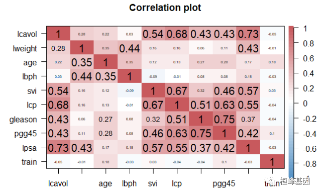
为了与主成分分析方法进行比较，我们仍然选择 prostate 这个数据集，suiran 只有97个观测共9个变量，但通过与传统技术比较，足以让我们掌握正则化技术。斯坦福大学医疗中心提供了97个病人的前列腺特异性抗原（PSA）数据，这些病人均接受前列腺根治切除术。我们的目标是，通过临床检测提供的数据建立一个预测模型预测患者术后PSA水平。对于患者在手术后能够恢复到什么程度，PSA水平可能是一个较为有效的预后指标。手术之后，医生会在各个时间区间检查患者的PSA水平，并通过各种公式确定患者是否康复。术前预测模型和术后数据（这里没有提供）互相配合，就可能提高前列腺癌诊疗水平，改善其预后。如下所示：

lcavol：肿瘤体积的对数值；

lweight：前列腺重量的对数值；

age：患者年龄（以年计）；

bph：良性前列腺增生（BPH）量的对数值，非癌症性质的前列腺增生；

svi：精囊是否受侵，一个指标变量，表示癌细胞是否已经透过前列腺壁侵入精囊腺（1—是， 0—否）；

lcp：包膜穿透度的对数值，表示癌细胞扩散到前列腺包膜之外的程度；

leason：患者的Gleason评分；由病理学家进行活体检查后给出（2—10） ，表示癌细胞的变异程度—评分越高，程度越危险；

pgg45：Gleason评分为4或5所占的百分比；

lpsa：PSA值的对数值，响应变量；

rain：一个逻辑向量（TRUE或FALSE，用来区分训练数据和测试数据）。

data(prostate)
str(prostate)
## 'data.frame':	97 obs. of  10 variables:
##  $ lcavol : num  -0.58 -0.994 -0.511 -1.204 0.751 ...
##  $ lweight: num  2.77 3.32 2.69 3.28 3.43 ...
##  $ age    : int  50 58 74 58 62 50 64 58 47 63 ...
##  $ lbph   : num  -1.39 -1.39 -1.39 -1.39 -1.39 ...
##  $ svi    : int  0 0 0 0 0 0 0 0 0 0 ...
##  $ lcp    : num  -1.39 -1.39 -1.39 -1.39 -1.39 ...
##  $ gleason: int  6 6 7 6 6 6 6 6 6 6 ...
##  $ pgg45  : int  0 0 20 0 0 0 0 0 0 0 ...
##  $ lpsa   : num  -0.431 -0.163 -0.163 -0.163 0.372 ...
##  $ train  : logi  TRUE TRUE TRUE TRUE TRUE TRUE ...
corPlot(prostate, gr = colorRampPalette(c("#2171B5", "white", "#B52127")))

3. 因子分析

我们举两个不同数据类型的例子，一类是常规临床数据，另一种是协方差数据，比较两中方式的优缺点。

a) 常规数据分析

首先判断需要提取的公共因子个数，函数 fa.parallel 可以判断需提取的因子个数。现在决定提取两个因子，可使用fa()函数获得相应的结果。fa()函数的格式如下: fa(r, nfactors=, n.obs=, rotate=, scores=, fm=)，其中:

1. r是相关系数矩阵或者原始数据矩阵;

2. nfactors设定提取的因子数(默认为1);

3. n.obs是观测数(输入相关系数矩阵时需要填写);

4. rotate设定旋转的方法(默认互变异数最小法);

5. scores设定是否计算因子得分(默认不计算);

6. fm设定因子化方法(默认极小残差法)。

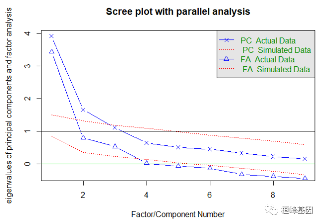
我们发现结果并不显著，那么我们需要对变量进行降维，也就是挑选对因变量起到更重要的变量，于是我们通过因子分析来获得影响大的因子，通过迭代的方式获得碎石图，首先判断因子的数目，这里使用Cattell碎石检验，表示了特征值与主成数目的关系。一般的原则是：要保留的因子的个数的特征值要大于0且大于平行分析的特征值，我们看到大于0的为3个特征，如下：

# Exploratory factor analysis of prostate data options(digits=2) determine
# number of factors to extract
fa.parallel(prostate[, -10], fa = "fa", n.obs = 97, n.iter = 100, show.legend = TRUE,
    main = "Scree plot with parallel analysis")
## Parallel analysis suggests that the number of factors =  3  and the number of components =  NA
abline(h = 0, lwd = 1, col = "green")

我们同时做主成分和因子分析，观察找到的主成分个数和因子个数都为3，其中主成分分析要求大于1的个数，而因子分析的个数要求大于0的个数，如下：

fa.parallel(prostate[, -10], fa = "both", n.obs = 97, n.iter = 100, show.legend = TRUE,
    main = "Scree plot with parallel analysis")
## Parallel analysis suggests that the number of factors =  3  and the number of components =  2
abline(h = 0, lwd = 1, col = "green")

探索性因子分析采用最小残差法和主轴法、加权最小二乘法或最大似然法进行因子分析,在潜变量探索性因子分析(EFA)的多种方法中，利用普通最小二乘(OLS)求最小残差(minres)解是较好的方法之一。这就产生了非常类似于最大似然的解，即使是对于行为不佳的矩阵。minres的一种变体是加权最小二乘(WLS)。也许最传统的技术是主轴(PAF)。对相关矩阵进行特征值分解，然后用前n个因子估计每个变量的共同性。这些共同性输入到对角线上，重复这个过程，直到和(diag)不变化。另一种估计方法是最大似然法。对于性能良好的矩阵，最大似然因子分析(fa或facal函数)可能是首选。用fa和n.iter >求得了载荷和因子间相关性的Bootstrapped置信区间。

fa <- fa(prostate[, -10], nfactors = 3, rotate = "none", fm = "pa")
fa
## Factor Analysis using method =  pa
## Call: fa(r = prostate[, -10], nfactors = 3, rotate = "none", fm = "pa")
## Standardized loadings (pattern matrix) based upon correlation matrix
##          PA1   PA2   PA3   h2   u2 com
## lcavol  0.78 -0.01 -0.27 0.68 0.32 1.2
## lweight 0.36  0.65 -0.12 0.57 0.43 1.6
## age     0.32  0.38  0.25 0.31 0.69 2.7
## lbph    0.15  0.64  0.20 0.47 0.53 1.3
## svi     0.67 -0.19 -0.25 0.55 0.45 1.5
## lcp     0.81 -0.23 -0.10 0.72 0.28 1.2
## gleason 0.67 -0.17  0.45 0.68 0.32 1.9
## pgg45   0.77 -0.20  0.45 0.83 0.17 1.8
## lpsa    0.77  0.17 -0.33 0.73 0.27 1.5
## 
##                        PA1  PA2  PA3
## SS loadings           3.60 1.16 0.77
## Proportion Var        0.40 0.13 0.09
## Cumulative Var        0.40 0.53 0.61
## Proportion Explained  0.65 0.21 0.14
## Cumulative Proportion 0.65 0.86 1.00
## 
## Mean item complexity =  1.6
## Test of the hypothesis that 3 factors are sufficient.
## 
## The degrees of freedom for the null model are  36  and the objective function was  4.37 with Chi Square of  403.19
## The degrees of freedom for the model are 12  and the objective function was  0.33 
## 
## The root mean square of the residuals (RMSR) is  0.03 
## The df corrected root mean square of the residuals is  0.05 
## 
## The harmonic number of observations is  97 with the empirical chi square  6.46  with prob <  0.89 
## The total number of observations was  97  with Likelihood Chi Square =  29.37  with prob <  0.0035 
## 
## Tucker Lewis Index of factoring reliability =  0.855
## RMSEA index =  0.122  and the 90 % confidence intervals are  0.067 0.18
## BIC =  -25.52
## Fit based upon off diagonal values = 0.99
## Measures of factor score adequacy             
##                                                    PA1  PA2  PA3
## Correlation of (regression) scores with factors   0.96 0.85 0.86
## Multiple R square of scores with factors          0.93 0.72 0.73
## Minimum correlation of possible factor scores     0.85 0.43 0.46
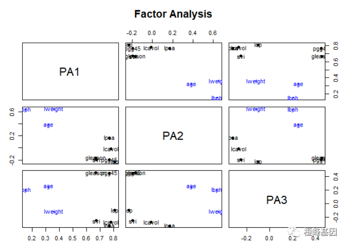
factor.plot(fa, labels = rownames(fa$loadings))

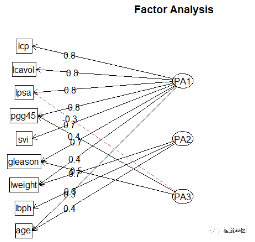
绘制因子载荷，如下

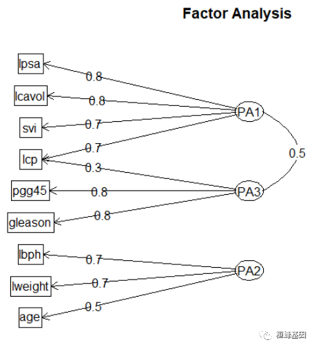
fa.diagram(fa, simple = FALSE)

因子旋转应不应该傲旋转? 旋转可以修改每个变量的载荷，这样有助于对因子的解释。旋转后的因子分能够解释的方差总量是不变的，但是每个因子对于能够解释的方差总量的贡献会改变。在旋转过程中，你会发现载荷的值或者更远离0，或者更接近0，这在理论上可以帮助我们识别那些对因子起重要作用的变量。这是一种将变量和唯一因子联系起来的尝试。请记住，因子分析是一种无监督学习，所以你是在努力去理解数据，而不是在验证某种假设。总之，旋转有助于你的这种努力。最常用的因子旋转方法被称为方差最大法。虽然还有其他方法，比如四次方最大法和等量最大法。但我们主要讨论方差最大旋转。根据我的经验，其他方法从来没有提供过比方差最大法更好的解。当然，你可以通过反复实验来决定使用哪种方法。在方差最大法中，我们要使平方后的载荷的总方差最火。方差最大化过程会旋转特征空间的特和坐标。但不改变致据点的也置。

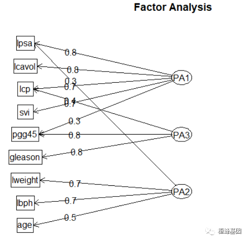
由输出结果可知，第一因子在6个观测变量上的载荷均较大，第二因子在lweight,lbph,这量个变量上载荷较大，第三个主成分影响都不大，载荷相对较小，但相差不大。两主成分解释了该数据的73%，但该结果并不便于解释三个因子。因此，考虑进行正交选择提取因子。

# Listing 14.7 - Factor extraction with orthogonal rotation
fa.varimax <- fa(prostate[, -10], nfactors = 3, rotate = "varimax", fm = "pa")
fa.varimax
## Factor Analysis using method =  pa
## Call: fa(r = prostate[, -10], nfactors = 3, rotate = "varimax", fm = "pa")
## Standardized loadings (pattern matrix) based upon correlation matrix
##           PA1   PA3   PA2   h2   u2 com
## lcavol   0.78  0.23  0.15 0.68 0.32 1.2
## lweight  0.29 -0.09  0.69 0.57 0.43 1.4
## age      0.06  0.25  0.49 0.31 0.69 1.5
## lbph    -0.07  0.04  0.68 0.47 0.53 1.0
## svi      0.70  0.24 -0.05 0.55 0.45 1.2
## lcp      0.72  0.45 -0.02 0.72 0.28 1.7
## gleason  0.27  0.77  0.10 0.68 0.32 1.3
## pgg45    0.35  0.83  0.10 0.83 0.17 1.4
## lpsa     0.79  0.13  0.30 0.73 0.27 1.4
## 
##                        PA1  PA3  PA2
## SS loadings           2.52 1.69 1.32
## Proportion Var        0.28 0.19 0.15
## Cumulative Var        0.28 0.47 0.61
## Proportion Explained  0.46 0.31 0.24
## Cumulative Proportion 0.46 0.76 1.00
## 
## Mean item complexity =  1.3
## Test of the hypothesis that 3 factors are sufficient.
## 
## The degrees of freedom for the null model are  36  and the objective function was  4.37 with Chi Square of  403.19
## The degrees of freedom for the model are 12  and the objective function was  0.33 
## 
## The root mean square of the residuals (RMSR) is  0.03 
## The df corrected root mean square of the residuals is  0.05 
## 
## The harmonic number of observations is  97 with the empirical chi square  6.46  with prob <  0.89 
## The total number of observations was  97  with Likelihood Chi Square =  29.37  with prob <  0.0035 
## 
## Tucker Lewis Index of factoring reliability =  0.855
## RMSEA index =  0.122  and the 90 % confidence intervals are  0.067 0.18
## BIC =  -25.52
## Fit based upon off diagonal values = 0.99
## Measures of factor score adequacy             
##                                                    PA1  PA3  PA2
## Correlation of (regression) scores with factors   0.92 0.91 0.84
## Multiple R square of scores with factors          0.84 0.82 0.71
## Minimum correlation of possible factor scores     0.67 0.65 0.42

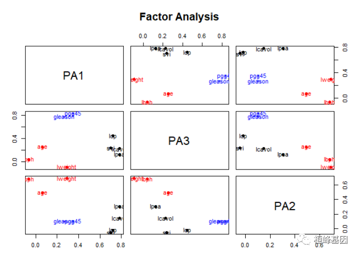
绘制因子/集群加载，并根据它们的最高加载将项目分配给集群,如下：

# plot factor solution
factor.plot(fa.varimax, labels = rownames(fa.varimax$loadings))

绘制旋转后的因子载荷，如下

fa.diagram(fa.varimax, simple = FALSE)

b) 协方差数据的因子分析

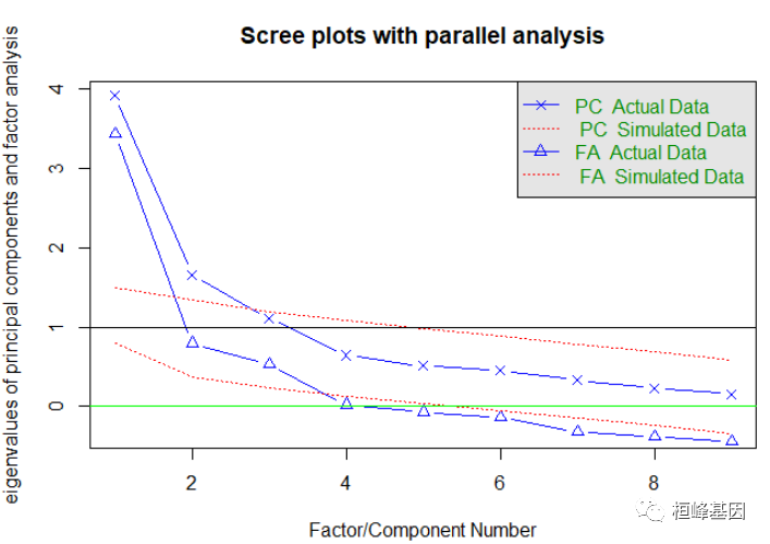
我们先计算 prostate 数据集的协方差，然后判断提取因子个数，我们看到结果同时展示了PCA和EFA的结果。PCA结果建议提取两个或者三个成分，EFA建议提取3个因子。注意,代码中使用了fa=“both”，因子图形将会同时展示主成分和公共因子分析的结果。

p.cor = cor(prostate[, -10])
# convert covariances to correlations
correlations <- cov2cor(p.cor)
correlations
##            lcavol   lweight       age         lbph         svi          lcp
## lcavol  1.0000000 0.2805214 0.2249999  0.027349703  0.53884500  0.675310484
## lweight 0.2805214 1.0000000 0.3479691  0.442264395  0.15538491  0.164537146
## age     0.2249999 0.3479691 1.0000000  0.350185896  0.11765804  0.127667752
## lbph    0.0273497 0.4422644 0.3501859  1.000000000 -0.08584324 -0.006999431
## svi     0.5388450 0.1553849 0.1176580 -0.085843238  1.00000000  0.673111185
## lcp     0.6753105 0.1645371 0.1276678 -0.006999431  0.67311118  1.000000000
## gleason 0.4324171 0.0568821 0.2688916  0.077820447  0.32041222  0.514830063
## pgg45   0.4336522 0.1073538 0.2761124  0.078460018  0.45764762  0.631528246
## lpsa    0.7344603 0.4333194 0.1695928  0.179809404  0.56621822  0.548813175
##            gleason      pgg45      lpsa
## lcavol  0.43241706 0.43365225 0.7344603
## lweight 0.05688210 0.10735379 0.4333194
## age     0.26889160 0.27611245 0.1695928
## lbph    0.07782045 0.07846002 0.1798094
## svi     0.32041222 0.45764762 0.5662182
## lcp     0.51483006 0.63152825 0.5488132
## gleason 1.00000000 0.75190451 0.3689868
## pgg45   0.75190451 1.00000000 0.4223159
## lpsa    0.36898681 0.42231586 1.0000000
# 判断需要提取的公共因子个数 determine number of factors to extract
fa.parallel(correlations, n.obs = 97, fa = "both", n.iter = 100, main = "Scree plots with parallel analysis")
## Parallel analysis suggests that the number of factors =  3  and the number of components =  2
abline(h = 0, lwd = 1, col = "green")

后续的分析都与上面的一致，因子旋转，如下：

# Listing 14.6 - Principal axis factoring without rotation
fa <- fa(correlations, nfactors = 3, rotate = "none", fm = "pa")
fa
## Factor Analysis using method =  pa
## Call: fa(r = correlations, nfactors = 3, rotate = "none", fm = "pa")
## Standardized loadings (pattern matrix) based upon correlation matrix
##          PA1   PA2   PA3   h2   u2 com
## lcavol  0.78 -0.01 -0.27 0.68 0.32 1.2
## lweight 0.36  0.65 -0.12 0.57 0.43 1.6
## age     0.32  0.38  0.25 0.31 0.69 2.7
## lbph    0.15  0.64  0.20 0.47 0.53 1.3
## svi     0.67 -0.19 -0.25 0.55 0.45 1.5
## lcp     0.81 -0.23 -0.10 0.72 0.28 1.2
## gleason 0.67 -0.17  0.45 0.68 0.32 1.9
## pgg45   0.77 -0.20  0.45 0.83 0.17 1.8
## lpsa    0.77  0.17 -0.33 0.73 0.27 1.5
## 
##                        PA1  PA2  PA3
## SS loadings           3.60 1.16 0.77
## Proportion Var        0.40 0.13 0.09
## Cumulative Var        0.40 0.53 0.61
## Proportion Explained  0.65 0.21 0.14
## Cumulative Proportion 0.65 0.86 1.00
## 
## Mean item complexity =  1.6
## Test of the hypothesis that 3 factors are sufficient.
## 
## The degrees of freedom for the null model are  36  and the objective function was  4.37
## The degrees of freedom for the model are 12  and the objective function was  0.33 
## 
## The root mean square of the residuals (RMSR) is  0.03 
## The df corrected root mean square of the residuals is  0.05 
## 
## Fit based upon off diagonal values = 0.99
## Measures of factor score adequacy             
##                                                    PA1  PA2  PA3
## Correlation of (regression) scores with factors   0.96 0.85 0.86
## Multiple R square of scores with factors          0.93 0.72 0.73
## Minimum correlation of possible factor scores     0.85 0.43 0.46

# Listing 14.7 - Factor extraction with orthogonal rotation
fa.varimax <- fa(correlations, nfactors = 3, rotate = "varimax", fm = "pa")
fa.varimax
## Factor Analysis using method =  pa
## Call: fa(r = correlations, nfactors = 3, rotate = "varimax", fm = "pa")
## Standardized loadings (pattern matrix) based upon correlation matrix
##           PA1   PA3   PA2   h2   u2 com
## lcavol   0.78  0.23  0.15 0.68 0.32 1.2
## lweight  0.29 -0.09  0.69 0.57 0.43 1.4
## age      0.06  0.25  0.49 0.31 0.69 1.5
## lbph    -0.07  0.04  0.68 0.47 0.53 1.0
## svi      0.70  0.24 -0.05 0.55 0.45 1.2
## lcp      0.72  0.45 -0.02 0.72 0.28 1.7
## gleason  0.27  0.77  0.10 0.68 0.32 1.3
## pgg45    0.35  0.83  0.10 0.83 0.17 1.4
## lpsa     0.79  0.13  0.30 0.73 0.27 1.4
## 
##                        PA1  PA3  PA2
## SS loadings           2.52 1.69 1.32
## Proportion Var        0.28 0.19 0.15
## Cumulative Var        0.28 0.47 0.61
## Proportion Explained  0.46 0.31 0.24
## Cumulative Proportion 0.46 0.76 1.00
## 
## Mean item complexity =  1.3
## Test of the hypothesis that 3 factors are sufficient.
## 
## The degrees of freedom for the null model are  36  and the objective function was  4.37
## The degrees of freedom for the model are 12  and the objective function was  0.33 
## 
## The root mean square of the residuals (RMSR) is  0.03 
## The df corrected root mean square of the residuals is  0.05 
## 
## Fit based upon off diagonal values = 0.99
## Measures of factor score adequacy             
##                                                    PA1  PA3  PA2
## Correlation of (regression) scores with factors   0.92 0.91 0.84
## Multiple R square of scores with factors          0.84 0.82 0.71
## Minimum correlation of possible factor scores     0.67 0.65 0.42

斜交旋转提取因子，获得结果明显比正交旋转的效果更好，如下：

# Listing 14.8 - Factor extraction with oblique rotation
# install.packages('GPArotation')
library(GPArotation)
fa.promax <- fa(correlations, nfactors = 3, rotate = "promax", fm = "pa")
fa.promax
## Factor Analysis using method =  pa
## Call: fa(r = correlations, nfactors = 3, rotate = "promax", fm = "pa")
## Standardized loadings (pattern matrix) based upon correlation matrix
##           PA1   PA3   PA2   h2   u2 com
## lcavol   0.80  0.03  0.04 0.68 0.32 1.0
## lweight  0.29 -0.22  0.68 0.57 0.43 1.6
## age     -0.06  0.24  0.49 0.31 0.69 1.5
## lbph    -0.15  0.03  0.71 0.47 0.53 1.1
## svi      0.72  0.08 -0.15 0.55 0.45 1.1
## lcp      0.68  0.30 -0.13 0.72 0.28 1.5
## gleason  0.05  0.79  0.04 0.68 0.32 1.0
## pgg45    0.12  0.83  0.02 0.83 0.17 1.0
## lpsa     0.82 -0.10  0.21 0.73 0.27 1.2
## 
##                        PA1  PA3  PA2
## SS loadings           2.58 1.66 1.29
## Proportion Var        0.29 0.18 0.14
## Cumulative Var        0.29 0.47 0.61
## Proportion Explained  0.47 0.30 0.23
## Cumulative Proportion 0.47 0.77 1.00
## 
##  With factor correlations of 
##      PA1  PA3  PA2
## PA1 1.00 0.51 0.25
## PA3 0.51 1.00 0.18
## PA2 0.25 0.18 1.00
## 
## Mean item complexity =  1.2
## Test of the hypothesis that 3 factors are sufficient.
## 
## The degrees of freedom for the null model are  36  and the objective function was  4.37
## The degrees of freedom for the model are 12  and the objective function was  0.33 
## 
## The root mean square of the residuals (RMSR) is  0.03 
## The df corrected root mean square of the residuals is  0.05 
## 
## Fit based upon off diagonal values = 0.99
## Measures of factor score adequacy             
##                                                    PA1  PA3  PA2
## Correlation of (regression) scores with factors   0.94 0.93 0.85
## Multiple R square of scores with factors          0.89 0.87 0.73
## Minimum correlation of possible factor scores     0.78 0.74 0.45

# calculate factor loading matrix
fsm <- function(oblique) {
    if (class(oblique)[2] == "fa" & is.null(oblique$Phi)) {
        warning("Object doesn't look like oblique EFA")
    } else {
        P <- unclass(oblique$loading)
        F <- P %*% oblique$Phi
        colnames(F) <- c("PA1", "PA2", "PA3")
        return(F)
    }
}
fsm(fa.promax)
##                PA1        PA2        PA3
## lcavol  0.82473291 0.44227350 0.24555125
## lweight 0.34220476 0.04243046 0.70717334
## age     0.18477222 0.29736739 0.51524467
## lbph    0.03268287 0.07473469 0.67218104
## svi     0.72626068 0.41757206 0.04449359
## lcp     0.79912417 0.62091939 0.08992345
## gleason 0.45900614 0.82088146 0.18990904
## pgg45   0.55288520 0.90185461 0.20082633
## lpsa    0.82381653 0.35706958 0.39508870

# factor scores
fa.promax$weights
##                  PA1         PA3         PA2
## lcavol   0.243980481  0.05617920  0.03965284
## lweight  0.063289015 -0.05858661  0.42084810
## age      0.001136759  0.04500146  0.19707194
## lbph    -0.052983656  0.03009248  0.37132673
## svi      0.161318100  0.01106634 -0.08257798
## lcp      0.299975224  0.08308988 -0.12679762
## gleason -0.015790579  0.30869180  0.04827821
## pgg45    0.041112967  0.62164473  0.07257584
## lpsa     0.359024621 -0.10014835  0.15129501

我们看因子的解决方案，如下：

# plot factor solution
factor.plot(fa.promax, labels = rownames(fa.promax$loadings))

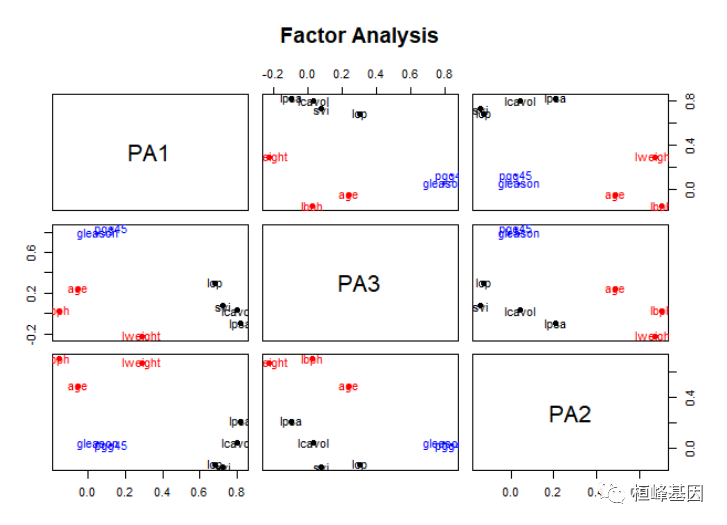
获得的因子分析结果，跟常规临床数据比较，我们发现使用斜交转轴法的结果更清晰，根据符合我们的预期，如下：

fa.diagram(fa.promax, simple = FALSE)

对因子分析非常有用的软件包，FactoMineR包不仅提供了PCA和EFA方法，还包含潜变量模型。FAiR包使用遗传算法来估计因子分析模型，增强了模型参数估计能力，能够处理不等式的约束条件。GPArotation包提供了许多因子旋转方法；nFactors包提供了用来判断因子数目方法。

其他相关方法

先验知识的模型：先从一些先验知识开始，比如变量背后有几个因子、变量在因子上的载荷是怎样的、因子间的相关性如何，然后通过收集数据检验这些先验知识。这种方法称作验证性因子分析（CFA）。做CFA的软件包：sem、openMx和lavaan等。ltm包可以用来拟合测验和问卷中各项目的潜变量模型。潜类别模型（潜在的因子被认为是类别型而非连续型）可通过FlexMix、lcmm、randomLCA和poLC包进行拟合。lcda包可做潜类别判别分析，而lsa可做潜在语义分析----一种自然语言处理中的方法。ca包提供了可做简单和多重对应分析的函数。R中还包含了众多的多维标度法（MDS）计算工具。

1. MDS即可用发现解释相似性和可测对象间距离的潜在维度;

2. cmdscale（）函数可做经典的MDS;

3. MASS包中的isoMDS（）函数可做非线性MDS;

4. vagan包中则包含了两种MDS的函数。

References:

1. Floyd, Frank J. and Widaman, Keith. F (1995) Factor analysis in the development and refinement of clinical assessment instruments. Psychological Assessment, 7(3):286-299, 1995.

2. Horn, John (1965) A rationale and test for the number of factors in factor analysis. Psychometrika, 30, 179-185.

3. Humphreys, Lloyd G. and Montanelli, Richard G. (1975), An investigation of the parallel analysis criterion for determining the number of common factors. Multivariate Behavioral Research, 10, 193-205.

4. Revelle, William and Rocklin, Tom (1979) Very simple structure - alternative procedure for estimating the optimal number of interpretable factors. Multivariate Behavioral Research, 14(4):403-414.

5. Velicer, Wayne. (1976) Determining the number of components from the matrix of partial correlations. Psychometrika, 41(3):321-327, 1976.