准备写这篇的时候，刚好在放孤勇者~
我们争取雁过留痕，把前段时间的尝试都写下来吧

这个比赛可能有一点点特殊，为了让大家更好地测试，补充数据集里放了预测时间段内的数据，所以存在数据泄露的问题现在排行榜上的排名是大家为了好玩儿用泄露数据做出来的

目前，我看到的没有用数据泄露的分享基本0.3多的已经很少了，可以等10月份比赛结束后，再看一下高分方案。

赛题链接↓↓↓(数据下载地址都在链接里可以找到)：
https://www.kaggle.com/competitions/jpx-tokyo-stock-exchange-prediction

目录

1.赛题解析

1.1 基本信息介绍

日本交易所JPX举办，要求根据日本市场的金融数据进行建模，预测模型训练完成后一段时间段内的真实收益情况。

1.2 提供数据(赛题输入)

数据文件夹：

文件夹	内容描述
data_specifications	各字段的介绍
jpx_tokyo_market_prediction	启用 API 的文件。预计 API 将在五分钟内交付所有行并保留少于 0.5 GB 的内存
train_files	涵盖主要培训期的数据文件夹
supplemental_files	补充数据文件夹，包含补充训练数据的动态窗口。这将在 5 月初、6 月初以及提交被锁定前大约一周的比赛主要阶段使用新数据进行更新。
example_test_files	涵盖公共测试期间的数据文件夹。旨在促进离线测试

主要查看train_data训练数据文件夹下数据的基本信息

stock_prices.csv

stock_prices的列名对照

column_name	中文释义
RowId	记录的唯一id，由日期和证券代码组合而成
Date	交易日期
SecuritiesCode	当地证券代码
open	开盘价
High	当天最高价
Low	当天最低价
Close	收盘价
Volumn	成交量
AdjustmentFactor	调整因子
ExpectedDividend	预期股利
SupervisionFlag	受监管证券和拟退市证券的标志
Target	调整后的收盘价在 t+2 和 t+1 之间的变化率，其中 t+0 是交易日期。

其它表我没大用上，当时查了相关字段的信息放在这里吧
链接（后面放上来）

1.3 提交结果(赛题输出)

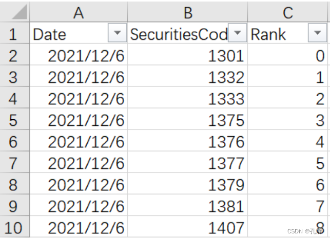
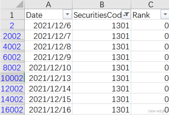
根据example_test_files文件夹中的提交示例文档sample_submission.csv可以看出，提交的结果为给定日期内，每天对2000只股票的排名。


那么，排名是如何生成的呢？
接口介绍文档中，可以看到给出的竞赛指标
[外链图片转存失败,源站可能有防盗链机制,建议将图片保存下来直接上传(img-LwbnIOTR-1658224070671)(en-resource://database/64690:1)]
这里的C(k,t)是第t天的收盘价，则r(k,t)(也就是我们训练数据中的target)是根据 ((t+2天的收盘价) - (t+1天的收盘价))÷(t+1天的收盘价) 计算出来的

我们可以对照训练数据计算一下target（ You can calculate the Target column from the Close column; it’s the return from buying a stock the next day and selling the day after that. ）

# 读取stock_price部分数据，看一下
df_price = pd.read_csv(f"{
      train_files_dir}/stock_prices.csv",nrows=10000)

df_need = df_price[df_price["SecuritiesCode"]==1301][["RowId","SecuritiesCode","Close","Target"]]

df_need["Close_shift1"] = df_need["Close"].shift(-1)   
df_need["Close_shift2"] = df_need["Close"].shift(-2)
df_need["rate"] = (df_need["Close_shift2"] - df_need["Close_shift1"]) / df_need["Close_shift1"]

可以看到我们这里计算的r(k,t)等于给出的target。

我们这里计算的利润即为假定明天买入，后天卖出。我们相当于计算的是每天的target。
target和当天之后，第二天、第三天的close价格相关。
预测的时候，每次只给出当天的数据，预测target并对当天的target值进行排名。

注意，rank是0-1999，不是1-2000.

1.4 评估依据

后面这部分是我们成绩的评判依据，我们只要根据上面的格式将每日排名进行提交，后面这部分通过调接口实现(防止使用预测时间后面的数据进行计算)。

提交的结果是根据每日收益的夏普比率来评估的。

The returns for a single day treat the 200 highest (e.g. 0 to 199) ranked stocks as purchased and the lowest (e.g. 1999 to 1800) ranked 200 stocks as shorted.

（每日的收益是将排名前200的股票视为买入，排名后200的股票视为卖出）
The stocks are then weighted based on their ranks and the total returns for the portfolio are calculated assuming the stocks were purchased the next day and sold the day after that.

前两百和后两百的股票变化乘以线性权重之差（取前后200名的股票测试一下）



(后200名乘以对应权重)
前两百名target乘以权重-后两百名乘以权重，这计算的是每天的收益，最终我们评估的是一段时间内每日收益的平均值除以其这段时间每日收益的标准差。
[外链图片转存失败,源站可能有防盗链机制,建议将图片保存下来直接上传(img-t37eZJJE-1658224302871)(en-resource://database/64704:1)]
最终得分高的排名靠前。

2.探索性数据分析

这部分我主要做的股价部分的数据，另外几个数据集虽然字段名称翻译了，但主要含义我没太搞懂，也不知道怎么用，所以就没再做，后面看了下别人做的。

2.1 双变量分析

取了2021年一年的数据

import seaborn as sb
import matplotlib.pyplot as plt
from datetime import datetime


# 分时段跑数据吧，笔记本跑不敢跑
df_price2021 = df_price[df_price.Date>datetime.strptime('2021-01-01','%Y-%m-%d')]

# 图表矩阵
g = sb.PairGrid(data = df_price2021, vars = ['Open', 'High', 'Low','Close','Volume','Target'])
# g.map_diag(plt.hist) # 用map_diag把直方图放到对角线上，不然的话是一条直线散点图
g.map_offdiag(plt.scatter)

可以看出来：

• open，high，low，close价格之间的相关性很强
• 价格和交易量之间，交易量随价格的升高而快速降低，一般价格高的股票，交易量较低
• target成正态分布，相较于价格，target在交易量上的分布更加分散

各变量时间跨度上的分布状态(以2021年target出现了最大值的股票为例)

# 查看2021年最大target各字段在这一年中相对于时间的变化
SecuritiesCode2021_1 = df_price2021[df_price2021.Target == max(df_price2021.Target)].SecuritiesCode.item()
df_price2021_1 = df_price2021[df_price2021.SecuritiesCode==SecuritiesCode2021_1]
# price2021_1_timeseries = df_price2021_1.set_index("Date")  # (226, 11)
# 宽表变长表
df_price2021_2 = df_price2021_1[["Date",'Open', 'High', 'Low','Close']]
df_price2021_2 = df_price2021_2.set_index(["Date"])
df_price2021_3 = df_price2021_2.stack().reset_index()
df_price2021_3[0] = df_price2021_3[0].astype('float64')
df_price2021_3.Date = df_price2021_3.Date.apply(lambda x:mdates.date2num(x))   # 这里用datetime会报错
df_price2021_3.rename(columns={
    0:"value"},inplace = True)

# 多折线图
ax = sb.lineplot(data=df_price2021_3,x="Date",y="value",hue='level_1')
# get current axis
ax = plt.gca()
format_str = '%Y-%m-%d'
format_ = mdates.DateFormatter(format_str)
ax.xaxis.set_major_formatter(format_)
plt.xticks(rotation=15)
plt.show()

可以看出：

• 该股票在2021.8到2021.9期间出现过巨幅上升
• open，high，low，close的变化基本趋于一致

将股价，target，volume的时间变化曲线绘制到一起
可以使用函数封装一下绘制时间曲线的函数

# 打包时间序列折线图()
def time_line(df,col_li,time_col):
    '''
    this function is used to plot the trend of each variable over time
    :param df:dataframe,contains(
    :param col_li:variable list
    :param time_col:name of time column
    :return:figure
    '''
    # 宽表变长表
    df_price2021_2 = df_price2021_1[col_li+[time_col]]
    df_price2021_2 = df_price2021_2.set_index([time_col])
    df_price2021_3 = df_price2021_2.stack().reset_index()
    df_price2021_3[0] = df_price2021_3[0].astype('float64')
    df_price2021_3[time_col] = df_price2021_3[time_col].apply(lambda x: mdates.date2num(x))  # 这里用datetime会报错
    if len(col_li) == 1:
        y_name = col_li[0]
    else:
        y_name = "value"

    df_price2021_3.rename(columns={
    0: y_name}, inplace=True)

    # 长型数据多折线图
    if len(col_li) == 1:
        ax = sb.lineplot(data=df_price2021_3, x=time_col, y=y_name)
    else:
        ax = sb.lineplot(data=df_price2021_3, x=time_col,y=y_name, hue='level_1')
    # get current axis
    ax = plt.gca()
    format_str = '%Y-%m-%d'
    format_ = mdates.DateFormatter(format_str)
    ax.xaxis.set_major_formatter(format_)
    plt.xticks(rotation=15)
    plt.show()


# 画到一起去
plt.figure(figsize=[12,5])

plt.subplot(1,3,1)
time_line(df_price2021_1,['Open', 'High', 'Low','Close'],"Date")

plt.subplot(1,3,2)
time_line(df_price2021_1,["Target"],"Date")

plt.subplot(1,3,3)
time_line(df_price2021_1,["Volume"],"Date")

可以看到，

• target和股价变化趋势相近，均在21年8月多出现极为陡峭的峰值，但相比于股价，target的图像局部抖动更为剧烈
• 交易量volume也随股价波动，但在峰值处出现了一定的时间延后
  
  选取了2021年出现最低target的股票进行了分析：
• 可以看出在股价出现明显波动的地方，交易量也出现了较大的增长
• target在零值线附近波动，在股价明显波动时期，随之产生剧烈起伏

2.2 优秀EDA赏析

这篇是比较热门的eda notebook。
https://www.kaggle.com/code/abaojiang/jpx-detailed-eda

这篇主要是金融领域的特征工程汇总
https://www.kaggle.com/code/metathesis/feature-engineering-training-with-ta/notebook

3.尝试构建模型

3.1 LSTM

这里我们是先抽了一只股票做的预测，看一下预测效果。

# 导入需要的包
import pandas as pd
from sklearn.preprocessing import MinMaxScaler
import numpy as np
from keras.models import Sequential
from keras.layers import LSTM
from keras.layers import Dense, Dropout

加载数据

# set base_dir to load data
base_dir = r"D:/stock_data"

# train_data
train_files_dir = f"{
      base_dir}/train_files"

train_df = pd.read_csv(f"{
      base_dir}/train_files"+'/stock_prices.csv', parse_dates=True)  
valid_df = pd.read_csv(f"{
      base_dir}"+'/supplemental_files/stock_prices.csv', parse_dates=True)
train_df = pd.concat([train_df,valid_df])  # 这里是把训练数据和补充数据合并了，后面一起取了20％做测试
features = ['Open', 'High', 'Low', 'Close','Volume']

# 以code为1332的股票进行测试
prices = train_df.query("SecuritiesCode==1332")[features]

划分测试集

 test_split = round(len(prices)*0.2)  # 252

df_for_training = prices[:-252][features]   
print(df_for_training.shape)
df_for_training = df_for_training.dropna(how='any')
print(df_for_training.shape)
df_for_testing = prices[-252:][features]   

缩放数据

scaler = MinMaxScaler(feature_range=(0,1))   # 缩放数据
df_for_training_scaled = scaler.fit_transform(df_for_training)
df_for_testing_scaled = scaler.transform(df_for_testing)

生成训练数据、测试数据

# createXY
def createXY(dataset,n_past):
    dataX = []
    dataY = []
    for i in range(n_past, len(dataset)):
            dataX.append(dataset[i - n_past:i, 0:dataset.shape[1]])  # [0:30,0:5]  以0-29天的数据
            dataY.append(dataset[i,-2])    # 30  预测第30天的值
    return np.array(dataX),np.array(dataY)


# 生成数据
trainX,trainY=createXY(df_for_training_scaled,30)
# trainX.shape
testX,testY=createXY(df_for_testing_scaled,30)

keras进行回归预测

from keras.wrappers.scikit_learn import KerasRegressor   # keras进行回归预测
from sklearn.model_selection import GridSearchCV

grid_model = Sequential()
grid_model.add(LSTM(50,return_sequences=True,input_shape=(30,5)))
grid_model.add(LSTM(50))
grid_model.add(Dropout(0.2))
grid_model.add(Dense(1))    # 看一下keras各参数定义哈！！！

grid_model.compile(loss='mse',optimizer = 'adam')

history = grid_model.fit(trainX,trainY,epochs=10,batch_size=30,validation_data=(testX,testY))   # 拟合训练数据

画图看一下训练效果

from matplotlib import pyplot as plt
plt.plot(history.history['loss'],label='train')
plt.plot(history.history['val_loss'],label='test')
plt.legend()
plt.show()

进行预测，并对比真实数据查看效果

prediction=grid_model.predict(testX)

prediction_copies_array = np.repeat(prediction,5, axis=-1)

pred=scaler.inverse_transform(np.reshape(prediction_copies_array,(len(prediction),5)))[:,0]  # 逆变化，标准化后的数据转换为原始数据

# 真实数据
original_copies_array = np.repeat(testY,5, axis=-1)

# original_copies_array.shape

original=scaler.inverse_transform(np.reshape(original_copies_array,(len(testY),5)))[:,0]

绘图查看对比效果

plt.plot(original, color = 'red', label = 'Real  Stock Price')
plt.plot(pred, color = 'blue', label = 'Predicted  Stock Price')
plt.title(' Stock Price Prediction')
plt.xlabel('Time')
plt.ylabel(' Stock Price')
plt.legend()
plt.show()

• 以1332为例
  
• 以1377为列
  
  可以看出，预测结果和实际数据大致趋势吻合，但细小的抖动没有预测出来。而我们这次比赛主要看的就是每天价格波动产生的短期收益，所以要不然调节模型，让其可以尽可能地拟合出来这些扰动，然后以想办法准确预测后面两天股价为主，再来计算出来需要的target，要不然我们可以直接尝试预测target，后面尝试了下用sgbt直接预测target方法的可行性。

另：
lstm这里，下面这个人最后模拟出来的图我觉得还比较接近真实股价起伏，我只看了图，没复现，不知道实际效果，不知道展示的是不是他的最优效果，大家想了解的可以看一下https://www.kaggle.com/code/onurkoc83/multivariate-lstm-close-open-high-low-volume

3.2 Sgboost

看了大家在论坛里分享的案例，尝试直接用sgbt预测target。筛选部分特征进行改进，使用optuna进行调参，利用gpu加速，这个时候跑出来的最好结果可以达到0.297，再调整就怎么也上不去了。

# 导入对应模块
import os
import traceback
import numpy as np
import pandas as pd
import xgboost as xgb
from tqdm import tqdm
import jpx_tokyo_market_prediction
import warnings; warnings.filterwarnings("ignore")

prices1 = pd.read_csv("../input/jpx-tokyo-stock-exchange-prediction/train_files/stock_prices.csv",parse_dates=True)

# 选取2020年之后的prices数据
prices1 = prices1[prices1.Date>'2020-01-01']

prices = prices1.copy()
prices = prices.drop(["ExpectedDividend"],axis=1)

prices.isnull().sum()
prices = prices.dropna(how='any')
prices.isnull().sum()  # drop null values

# 获取各股票前一天的股价
cc = prices.groupby("SecuritiesCode").apply(lambda df: df['Close'].shift(1))
cc = pd.DataFrame(cc).reset_index(level=0)

prices = pd.merge(prices,cc['Close'],left_index=True,right_index=True)
prices.head()
prices.tail()

prices['delta'] = prices['Close_x'] - prices['Close_y']

# 查看是涨是跌
def getadvance(x):
    ret = 0
    if x > 0:
        ret = 1
    return(ret)

prices['advance'] = list(map(getadvance, prices['delta']))

prices['Date'] = pd.to_datetime(prices['Date'], format = "%Y-%m-%d")

def get_month(dt):   # 获取月份
    x = dt.strftime("%m")
    return(x)

prices['Month'] =  list(map(get_month, prices['Date']))

prices.rename(columns={
    "Close_x":"Close"},inplace=True)
prices.head()

def upper_shadow(df):
    return df['High'] - np.maximum(df['Close'], df['Open'])

def lower_shadow(df):
    return np.minimum(df['Close'], df['Open']) - df['Low']

prices['Upper_Shadow'] = upper_shadow(prices)
prices['Lower_Shadow'] = lower_shadow(prices)

# 最终确定的特征
features = ['Open', 'High', 'Low', 'Close',
            'Volume', 'AdjustmentFactor', 'SupervisionFlag', 
            'delta', 'advance', 'Month','Upper_Shadow','Lower_Shadow']
            
prices = prices.dropna(how='any')
prices.isnull().sum()

del prices['Date']

# 转换为类别格式
def cat_col(data) :
    data['SecuritiesCode'] = data['SecuritiesCode'].astype('category')
    data['SupervisionFlag'] = data['SupervisionFlag'].astype('category')
    data['advance'] = data['advance'].astype('category')
    data['AdjustmentFactor'] = data['AdjustmentFactor'].astype('category')
    data['Month'] = data['Month'].astype('category')
    return data

prices = cat_col(prices)

X = prices[features]
y = prices['Target']

# optuna调参+训练模型
import optuna
def objectives(trial):
    param = {
    
        'tree_method':'gpu_hist',
        'lambda': trial.suggest_loguniform('lambda', 1e-3, 10.0),
        'subsample': trial.suggest_categorical('subsample', [0.4,0.6,0.8,1.0]),
        'colsample_bytree': trial.suggest_categorical('colsample_bytree', [0.3,0.5,0.7,0.9,1.0]),
        'learning_rate': trial.suggest_categorical('learning_rate', [0.008,0.01,0.02,0.05]),
        "n_estimators" : trial.suggest_int('n_estimators', 300, 1000),
        'max_depth': trial.suggest_categorical('max_depth', [5,9,13,15,17,20]),
        'random_state': trial.suggest_categorical('random_state', [24, 48,2020]),
        'min_child_weight': trial.suggest_int('min_child_weight', 1, 10)
    }
    model = xgb.XGBRegressor(**param, enable_categorical=True)  # , enable_categorical=True
    model.fit(X, y)
    score = model.score(X, y)
    return score
    

studyxgb = optuna.create_study(direction='maximize', sampler=optuna.samplers.RandomSampler(seed=0))
studyxgb.optimize(objectives, n_trials=5)

trial = studyxgb.best_trial
params_best = dict(trial.params.items())
print(params_best)
# params_best['random_seed'] = 0

model = xgb.XGBRegressor(**params_best,enable_categorical=True,tree_method='gpu_hist')  # xgb.XGBRegressor(**param, enable_categorical=True)

# 打印最佳参数
print('study.best_params:', studyxgb.best_trial.value)
print('Number of finished trials:', len(studyxgb.trials))
print('Best trial:', studyxgb.best_trial.params)
print('study.best_params:', studyxgb.best_params)

print(model.tree_method)

model.fit(X,y)
model.score(X,y)

提交

import jpx_tokyo_market_prediction
env = jpx_tokyo_market_prediction.make_env()
iter_test = env.iter_test()

all_data = prices1.copy()


# 获取前一天股价
def latest_close(SecuritiesCode,date):
    temp = all_data[all_data.SecuritiesCode==SecuritiesCode].sort_values(by=["Date"],ascending=False)
    temp = temp[temp.Date<=date]
    return temp.iloc[-1]['Close']
   
for (prices, options, financials, trades, secondary_prices, sample_prediction) in iter_test:
#     print(prices)
#     del prices['Date']
#     print(prices)
#     qq = prices
    all_data = pd.concat([all_data,prices])
#     prices["Avg"] = sample_prediction["SecuritiesCode"].apply(get_avg)

    prices['Close_y'] = prices.apply(lambda x:latest_close(x.SecuritiesCode,x.Date),axis=1)
    prices['delta'] = prices['Close'] - prices['Close_y']
    prices['advance'] = list(map(getadvance, prices['delta']))
    prices['Date'] = pd.to_datetime(prices['Date'], format="%Y-%m-%d")
    prices['Month'] = list(map(get_month, prices['Date']))

    prices = cat_col(prices)
    prices['Date'] = prices['Date'].dt.strftime("%Y%m%d").astype(int)
    prices['Upper_Shadow'] = upper_shadow(prices)
    prices['Lower_Shadow'] = lower_shadow(prices)
    
    securities = prices["SecuritiesCode"]
    prices = prices[features]
    print('-------------------------------prices------------------------------')
    print(prices)
    print('------------------------------------------------------------------------------')

    sample_prediction["Prediction"] = model.predict(prices)
#     sample_prediction['SecuritiesCode'] = securities
    print('-------sample_prediction--------')
    print(sample_prediction)
    sample_prediction = sample_prediction.sort_values(by="Prediction", ascending=False)
    sample_prediction.Rank = np.arange(0, 2000)
    sample_prediction = sample_prediction.sort_values(by="SecuritiesCode", ascending=True)
    sample_prediction.drop(["Prediction"], axis=1)
    submission = sample_prediction[["Date", "SecuritiesCode", "Rank"]]
    print('-------------------------------submission------------------------------')
    print(submission)
    print('------------------------------------------------------------------------------')
    env.predict(submission)

3.3 其他尝试

3.3.1 短时间拟合预测

前面用lstm预测股价，更简单粗暴的方法是尝试用近3天或者近2天的时间推测后面两天的股价，做一个大致的估计。
代码片段

# 拟合后面两天的股价
df.Date = pd.to_datetime(df.Date, format="%Y-%m-%d")
df = df.set_index(['Date'])
df['day3'] = df.Close.rolling(window=3).apply(lambda y:
           np.poly1d(np.polyfit([0,1,2],y,1))(3),raw=True)
df['day2'] = df.Close.rolling(window=2).apply(lambda y:
           np.poly1d(np.polyfit([0,1],y,1))(2),raw=True)
df.reset_index()

这个方法效果还可以，分数大概可以跑到0.11-0.14左右。

3.3.2 Prophet

再后面主要是想把xgboost的结果提升一点儿，看别人添加其它特征的效果也不是很理想https://www.kaggle.com/code/junjitakeshima/jpx-add-new-features-eng。
于是，就开始考虑可以把prophet和sgboost做个结合，看一下效果怎么样(痛苦地开始……hhhh)。
主要是参考的这篇文章


然后，在做的时候大部分时间就转移到了
解决pystan的安装问题(改天可以专门放一篇博客出来)
解决用prophet时，pystan的打印太长问题……(prophet的使用和打印问题改天也一定会放上来的！！！)
调整代码，解决2000只股票预测内存不足以及时间太长会超过kaggle时间限制的问题……

这个尝试最终的效果并不理想，prophet我用的并不熟练，后面也没有时间调了。我会把部分代码放在下面，大家可以看看有没有什么想法优化一下。

# prophet部分
# import prophet
from prophet import Prophet
from prophet.make_holidays import make_holidays_df
import logging
logging.getLogger('prophet').setLevel(logging.WARNING)

# 设置pystan打印
class suppress_stdout_stderr(object):
    '''
    A context manager for doing a "deep suppression" of stdout and stderr in
    Python, i.e. will suppress all print, even if the print originates in a
    compiled C/Fortran sub-function.
       This will not suppress raised exceptions, since exceptions are printed
    to stderr just before a script exits, and after the context manager has
    exited (at least, I think that is why it lets exceptions through).

    '''
    def __init__(self):
        # Open a pair of null files
        self.null_fds = [os.open(os.devnull, os.O_RDWR) for x in range(2)]
        # Save the actual stdout (1) and stderr (2) file descriptors.
        self.save_fds = (os.dup(1), os.dup(2))

    def __enter__(self):
        # Assign the null pointers to stdout and stderr.
        os.dup2(self.null_fds[0], 1)
        os.dup2(self.null_fds[1], 2)

    def __exit__(self, *_):
        # Re-assign the real stdout/stderr back to (1) and (2)
        os.dup2(self.save_fds[0], 1)
        os.dup2(self.save_fds[1], 2)
        # Close the null files
        os.close(self.null_fds[0])
        os.close(self.null_fds[1])

# 设置节日
year_list = [2017,2018,2019,2020, 2021, 2022]
holidays = make_holidays_df(year_list=year_list, country='JP')

# 因为节假日不交易，所以节假日按真实日期算出来全为0，所以下面的日期先统一减了1天进行尝试
from datetime import timedelta
holidays['ds'] = holidays['ds'].apply(lambda x:x - timedelta(days=1))

# prophet预测
def run_prophet(tr):
#     tr = tr[["Date","Target"]]
#     tr.rename(columns={'Target': 'y', 'Date': 'ds'}, inplace=True)
    m = Prophet(holidays=holidays,
                daily_seasonality=False,
                changepoint_prior_scale=0.01)
    with suppress_stdout_stderr():
        m.fit(tr)
    return m


# 添加的特征
add_features = ['trend', 'yhat_lower', 'yhat_upper', 'trend_lower', 'trend_upper', 'additive_terms', 'additive_terms_lower', 'additive_terms_upper', 'holidays']

# 为每一组data创建一个prophet
from tqdm import tqdm
pbar = tqdm(total=2000)
count = 0
forecast_all = pd.DataFrame()
for cod in cod_list:
#     print(cod)
    names1 = globals()
    temp = names['cod_'+str(cod)][["Date","Target"]]
    temp.rename(columns={
    'Target': 'y', 'Date': 'ds'}, inplace=True)
    names1['m_'+str(cod)] = run_prophet(temp)
    new_feature = names1['m_'+str(cod)].predict(temp.drop('y', axis=1))
    names['cod_'+str(cod)] = pd.concat([names['cod_'+str(cod)],new_feature[add_features]],axis=1)  # 生成训练数据集的新特征
    # 向后预测一段时间
    future = names1['m_'+str(cod)].make_future_dataframe(periods=120)
    forecast = names1['m_'+str(cod)].predict(future)       # 存储预测特征，将来用来检索
#     print(forecast[add_features])
    forecast = forecast[add_features+['ds']]
    forecast['SecuritiesCode'] = cod
    forecast_all = pd.concat([forecast_all,forecast],axis = 0)
    del names1['m_'+str(cod)]
    count += 1
    if count == 200:
        pbar.update(200)
        count = 0
pbar.close()

prophet部分代码主要如上所示，其余部分还是按照上面sgbt的方法进行的计算，相当于在原有feature上添加了add_features部分。完整代码见git(链接)。

3.4 最终方案

最后的提交方案还是回到最开始跑到0.297的sgbt模型，处理了空值及价格调整部分，结果一下子就到了0.332。
价格调整是根据AdjustmentFactor这个字段，我们可以选择一个出现AdjustmentFactor不为1的股票进行查看。

prices[prices.SecuritiesCode==3176].head(25) #.query("AdjustmentFactor!=1")

调整代码

# 调整价格def adjust_price(price):
    from decimal import ROUND_HALF_UP, Decimal

    pcols = ["Open", "High", "Low", "Close"]

#     price.ExpectedDividend.fillna(0, inplace=True)

    def qround(x):
        return float(Decimal(str(x)).quantize(Decimal('0.1'), rounding=ROUND_HALF_UP))

    def adjust_prices(df):
        df = df.sort_values("Date", ascending=False)
        df.loc[:, "CumAdjust"] = df["AdjustmentFactor"].cumprod()

        # generate adjusted prices
        for p in pcols:
            df.loc[:, p] = (df["CumAdjust"] * df[p]).apply(qround)
        df.loc[:, "Volume"] = df["Volume"] / df["CumAdjust"]
        df.ffill(inplace=True)  # 去除空值了
        df.bfill(inplace=True)

        # generate and fill Targets
        # df.loc[:, "Target"] = df.Close.pct_change().shift(-2).fillna(df.Target).fillna(0)
        df.Target.fillna(0, inplace=True)

        return df
    # generate Adjusted#     price = price.sort_values(["SecuritiesCode", "Date"])
    price = price.groupby("SecuritiesCode").apply(adjust_prices).reset_index(drop=True)
    price = price.sort_values("RowId")
    return price

调整后的结果为0.332

不知道最后能排第多少名，虽然目前我看到上0.3的方案不是很多，但因为我调prophet把提交次数用完了，所以最后要加supplement数据的时候，没办法修改了~(是可以直接送走的程度)

4.小结一下

1. 整个参赛过程还是很有价值的，自己查阅学习了不少东西，非常感谢论坛里活跃积极分享的小伙伴，和真的完整的参加了比赛，坚持到最后的我自己hhhh
2. 对于最后想尝试的结合prophet的方法，我觉得有机会还能再救一下，一个是查阅的文章中也是处理时间序列预测问题，效果说的应该是比较好的，看有没有可能可以先复现一下他的代码，再结合当前案例进行调试。
3. 再有一个就是，中间优秀eda分享那里有一个关于金融方面特征工程的汇总，我觉得可以参考那篇文章加一些特征，没准效果会好一点。
4. 对于kaggle还不是很熟悉，提交以及文件存储方面后面可以再多多尝试。
5. 目前就想到这些了，把最近的学到的东西先梳理完吧，谢谢还能看到这里的人
   (有没有小伙伴我们下次可以一起参赛呀，团队力量大嘛~~~ )

5.参考链接

https://www.kaggle.com/code/metathesis/feature-engineering-training-with-ta/notebook

https://www.kaggle.com/code/jiripodivin/supervised-stocks-eda-and-basic-pca

https://www.kaggle.com/code/abaojiang/jpx-detailed-eda

https://www.kaggle.com/code/genbufuthark/jpx-datafile-description-in-japanese

https://www.kaggle.com/code/chumajin/english-ver-easy-to-understand-the-competition

https://www.zhihu.com/search?q=%E5%A4%8F%E6%99%AE%E6%AF%94%E7%8E%87&utm_content=search_suggestion&type=content

https://www.kaggle.com/code/bowaka/jpx-buying-strategy-backtest

https://github.com/keras-team/keras/pull/13598/commits/c735ab5b89bbf935075c84aab3437468e1fe8245

https://www.kaggle.com/code/ikeppyo/examples-of-higher-scores-than-perfect-predictions这是一个高分技巧，通过降低每日利润的标准差来提高分数

https://www.kaggle.com/code/paulorzp/jpx-prophet-forecasting-rolling-regression

https://stackoverflow.com/questions/45551000/how-to-control-output-from-fbprophet

prophet官网链接：
https://facebook.github.io/prophet/docs/quick_start.html#python-api

https://www.geeksforgeeks.org/time-series-analysis-using-facebook-prophet/?ref=gcse

https://towardsdatascience.com/time-series-analysis-with-facebook-prophet-how-it-works-and-how-to-use-it-f15ecf2c0e3a

https://towardsdatascience.com/boost-your-time-series-forecasts-combining-gradient-boosting-models-with-prophet-features-8e738234ffd这个是结合prophet的文章